Some time ago I encountered a situation at work where I needed high-resolution real-time image encoding on a constrained device. My first suggestion was to use a temporal video codec (like H.264), but the customer wanted to be able to encode and decode still images independently. Since the platform had no hardware-accelerated encoder blocks and state-of-the-art compression algorithms like WebP and JPEG XL are CPU-bound and too slow for such an application, the only feasible solution was to fall back to a GPU-accelerated JPEG codec.
During this whole exercise, I realized that there is no GPU-accelerated implementation of the JPEG XL codec, and so I asked myself why not make one myself. This post is the answer to that question and the project (cujpegxl) that came out of it.
JPEG XL in a nutshell
JPEG XL is a compressed image format standardized in 2021-2022, based on two algorithms (FUIF and PIK) initially developed in 2015-2017. It supports both lossless and lossy compression, but my focus is primarily on the lossy one. The latter is a conceptual extension of JPEG compression, using a variable-block-size discrete cosine transform (VarDCT) in XYB colour space. At higher effort settings, the algorithm iteratively evaluates the Butteraugli distance between input and encoded image and uses it to tune the quantization settings. Another improvement over JPEG is the use of both Huffman and Asymmetric Numeral System (ANS) for entropy coding, letting the encoder pick the most suitable on a case-by-case basis.
The algorithm is standardized in ISO/IEC 18181, but an outline is available in freely accessible resources including the whitepaper [1] and the open-source reference implementation libjxl.
The algorithm is more complicated (and expensive) than JPEG and some parts of it require some effort to optimize for GPU execution, but overall it looked possible to get a GPU implementation going.
Algorithm anatomy
The JPEG XL algorithm has two main alternative frame coding methods, based on VarDCT (lossy) or on modular coding (can be lossless).1 In the following I focus on the lossy VarDCT path, which is the most relevant to my use case. The skeleton of the encoding algorithm is roughly the following:
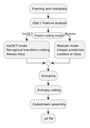
The algorithm starts by setting up the so-called codestream (i.e. the stream of encoded image data) with all metadata needed to render the image frames correctly. The word “frames” sounds confusing, but indeed JPEG XL supports multi-frame representation, even for still images, making the container quite flexible by allowing e.g. to store arbitrary channels with arbitrary semantics.
The encoder can then optionally perform a step to extract image features that can be encoded separately and then rendered on top of the decoded image, including patches of repeated image elements, splines of curvilinear features, and modelled intensity-dependent noise.
What comes next is the main part of the encoder. If we follow the VarDCT lossy branch, the key idea (compression in the frequency domain) is analogous to JPEG, but it is pushed way further. The image is first converted into XYB space2 to better exploit perceptual information, and is subjected to some preconditioning.3 The encoder then chooses a dynamic grid4 to partition the image into blocks. Unlike JPEG, which uses a fixed-size 8x8 grid, JPEG XL is allowed to use variable-sized blocks ranging from 2x2 to 256x256, allowing e.g. larger blocks to exploit flat regions, and smaller blocks to preserve details of more complex regions.
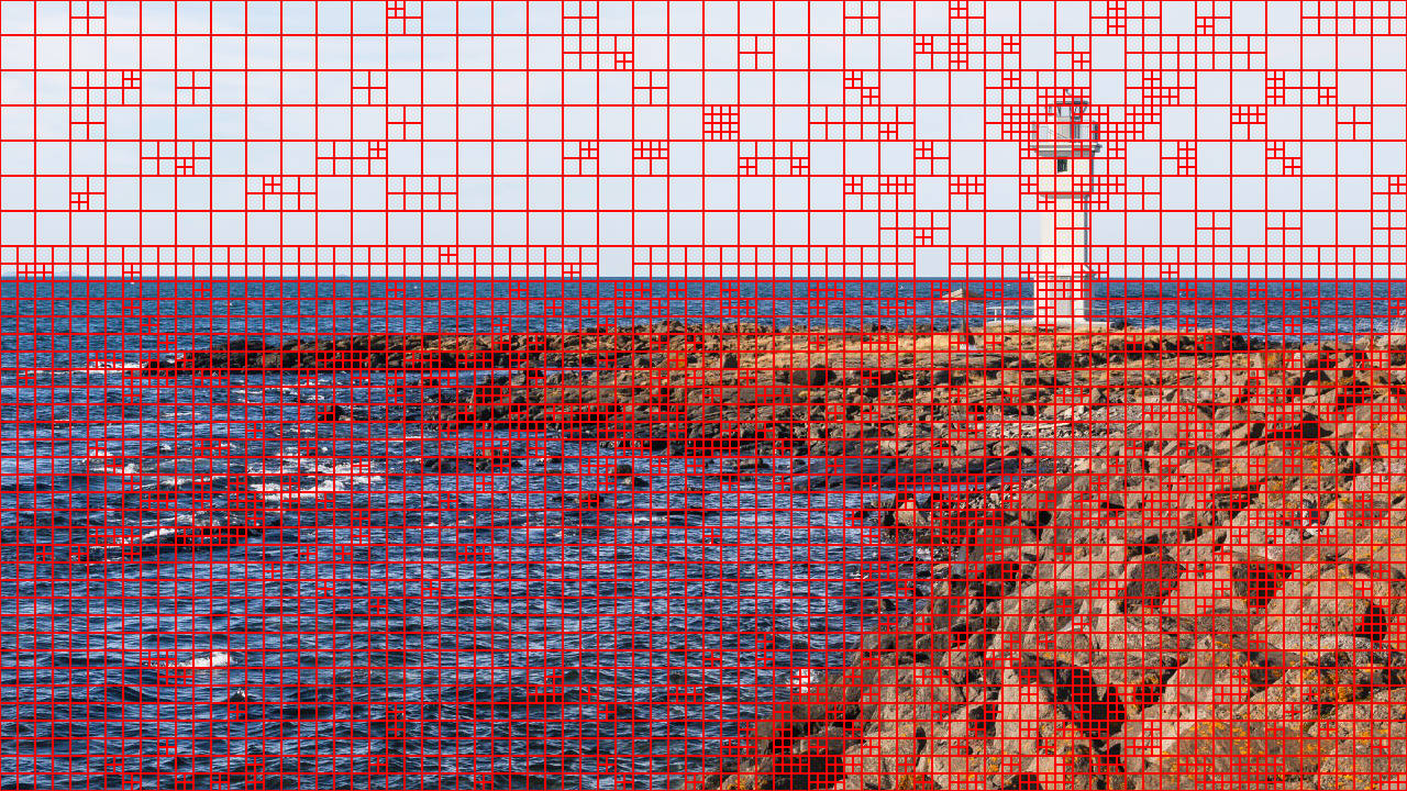 Example VarDCT grid selected by cujpegxl (720p) with 8 ≤ s ≤ 32.
Akranes lighthouse by Diego Delso on Wikimedia Commons, CC-BY-SA 4.0.

Blocks are then independently transformed with a discrete cosine transform. Like in JPEG, this allows to concentrate proportionally more information into low-frequency coefficients, allowing for more effective coding of the mostly small and low-entropy high-frequency coefficients.
Only the coefficients for the Y channel are effectively stored. The luminance channel encodes structural information and the chrominance is strongly correlated with it, so the X and B channels are reconstructed by predicting them with a simple linear transform from Y plus a residual (hence the name of chroma-from-luma prediction). If the prediction is good, the residuals will be small and therefore highly compressible.
Adaptive quantization is then performed on the coefficients. This is the real irreversible part that makes the algorithm truly lossy. Quantization is “adaptive” because it is weighted per transform \(t\), block \(b\), and channel \(c\), using both global information \(G\) and a per-block spatial field \(F_b\). A quantization of the \(k\)-th coefficient roughly looks like
\[q_{b,c,k} = \operatorname{round} \left( C_{b,c,k} \frac{G F_b}{W_{t,c,k}} \right) \\\]where \(\boldsymbol{W}\) is a weight matrix.5 The “step size” \(\Delta_{b,c,k} = \frac{W_{t,c,k}}{G F_b}\) roughly determines how lossy the quantization is.
A subsequent step organizes the encoded information to allow for efficient decoding. This step does not affect the image content but only the order in which the content itself is processed. Frames are divided into independent groups that can be processed in parallel in a progressive fashion. The DC coefficients6 are gathered in a low-frequency (LF) image at \(\frac{1}{8}\) of the resolution, and AC coefficients are organized in high-frequency (HF) passes that can be decoded progressively. In this fashion, the LF image alone provides a low-resolution preview of the whole image, and each HF pass adds more detail to it. This enables progressive and responsive image decoding from a still partially loaded/downloaded image, instead of a traditional monolithic decoding operation.
The last main algorithmic step is entropy coding, which provides lossless compression of the coefficients by deriving an optimal code to express them. While JPEG uses Huffman coding, JPEG XL uses both rANS and Huffman coding, choosing on a per-stream basis according to some heuristic, typically using Huffman coding for shorter streams (to avoid the overhead of rANS table construction), and rANS for larger streams where the higher compression rate makes a significant difference.
GPU notes
JPEG XL is overall less GPU friendly than JPEG. While the latter has a more regular, fixed-size grid, fixed quantization tables, and overall fewer dynamic/moving parts, JPEG XL has a variable size DCT grid that can cause uneven work and thread divergence, as well as spatially adaptive quantization with weights that change per channel and block. Entropy coding has a more complex histogram clustering, and rANS has a state that needs to be updated on every symbol. Transform selection, adaptive quantization, and perceptual optimizations involve many small decisions with irregular feedback loops.
While the bulk of image operations and filters can be mapped to GPU kernels, all this complexity makes it more challenging to come up with a well-optimized implementation that can effectively take advantage of the GPU architecture to its full extent. The task looked therefore non-trivial, but I decided to tackle it nonetheless.
Approach
JPEG XL is a fairly complex algorithm. A clean implementation would require months of developer work, and it would start with days of work just to read up and fully understand the algorithm. An interesting aspect of this project, however, is that there already is a complete open source reference implementation. This shifts the problem from a blank-slate implementation to primarily a CUDA port, and having a reference to both translate from and at the same time to be able to test against simplifies the problem significantly.
Given the complexity of the project, I used a mix of large models (GLM 5.3 and 5.2, GPT-5.6 Sol, Claude Opus 4.8), as with smaller models I have generally experienced their inability to properly deal with tasks of this complexity. Some people argue that larger models are only needed for the planning, and implementation can be delegated to smaller ones, but for tasks of this complexity, in my experience, implementation is also tricky and often smaller models cannot figure out solutions, when they don’t simply end up in a doom loop of bad decisions and become unable to make progress.
Prompting
This was nonetheless a large and complex software project, even for AI agents,7 and especially with an underspecified framing it would be hard for the AI to come up with a consistent implementation that solves the right problem. I approached the project through an initial planning session to define the scope and implementation milestones, and then proceeded with AI agents implementing the relevant steps in the roadmap graph, following the dependency order.
I used my typical AI coding approach by first having an agent define a high-level plan document specifying the goals (and non-goals), scope, constraints, requirements, and high-level milestone roadmap. This is accomplished by what in my skills I call an “inquisition”8 session, by having the agent relentlessly asking me questions until nothing is left ambiguous or unspecified.
Each milestone got in turn a dedicated document that specifies in more detail its scope, tasks, and exit criteria checklist. Each task can be implemented within an AI agent session, and each session ends by updating the status in the documents, so that the next fresh agent can pick up the next task directly. If a task ends up being too large or complex for a session, I let the agent write a handover document, so that a fresh agent can pick up the work by just reading it.
For this project, as I normally do for complex projects where I require high quality of the results, I reviewed the outcome of each task9 rather than letting the AI continue unsupervised for many tasks in a row, and I did not let the agents make key decisions autonomously, but rather instructed them to stop and ask for my input when a design decision or a key trade-off was needed. Even with a good plan, AI agents easily get off-track, and their bad decisions quickly compound, so early feedback is particularly useful to keep the project on track and avoid a lot of unnecessary work.10 This I think is more relevant for high-complexity projects, more mainstream software tasks are manageable by today’s AI agents in a more autonomous fashion.
Planning
I baked in the plan the key goals of my project:
- Conformance: the encoded images should be decodable by the reference
djxland by any conforming JPEG XL decoder. - Determinism: when encoding the same input on the same platform, output must be byte-identical.
- Performance: the encoder should use the GPU efficiently and meet real-time performance (≥ 15 fps @ 4K on low-end devices, ideally only using a slice of the resource budget).
I incorporated in the planning phase some critical scope and trade-off decisions. The JPEG XL algorithm is fairly complex and not all parts are easy to optimize on GPU. After basic work to establish an evaluation framework, build system scaffolding, and quality checks, the milestones started by first implementing a minimal conforming encoder, and alter iteratively adding to it more and more parts to improve compression rate and quality. Completeness of the JPEG XL algorithm is a non-goal and, due to the high performance runtime goal, parts can be omitted if they are too expensive and I conclude that they are not worth the quality/speed trade-off.
I also included some other scope limitations in the initial plan, for instance restricting support to 2160p/1080p/720p Y’UV 420 NV12 input. These constraints were aimed purely at speeding up the project ramp-up, by reducing the need for scaffolding and boilerplate for purely technical input/output marshalling, and can be very easily lifted later, after higher priority goals have been met.
Timeline
The first working encoder only implemented a fixed-size 8x8 DCT with a fixed quantization field. As one might imagine, this did not perform well in terms of image compression, but it produced a valid codestream that could be decoded with libjxl. Subsequent milestones added adaptive quantization, variable block size (to a limited set of sizes \(8 \le s \le 32\) that can be expanded later),11 chroma-from-luma prediction, and entropy optimization.
I interleaved the milestones with a few rounds of runtime optimization. AI agents tend to write poorly optimized code by default, and even when instructed with clear runtime goals, they tend to require some iterations to actually drop naive solutions and write more optimized code.12 One of the benefits of AI-generated code is that it is much easier to achieve optimizations such as kernel fusion, which is code-heavy and would be much more annoying to handwrite (and then maintain). In this project I fused the whole image front-end into a large kernel, which on top of allowing some compute savings has the benefit of substantially reducing DRAM traffic by skipping intermediate stores.
The first complete and functional version took just about a calendar week of weekend-and-evenings (after)work, to which I added a few more evenings of cleanup and optimizations. Something like this would have been impossible to accomplish in such a short timespan without AI; a work package of this size would have definitely been in the order of several developer-months FTE.
Some additions proved to be too expensive in terms of quality-speed trade-off and were therefore rejected. An example is rANS coding: the AIs struggled to come up with a fast-enough implementation either in pure GPU form13 or in a pipelined CPU-GPU hybrid. I am planning to come back to rANS coding in a later iteration, with a narrower and better-specified scope and closer human feedback, to see if I can get the AI to produce a more sustainable implementation.
Evaluation
Before even starting any work on feature implementation, the very first thing I set up was a framework for evaluation, creating a tool that takes as input a manifest with a collection of input images, runs compression and decompression, and evaluates compression loss using a few different metrics. PSNR is not particularly representative of perceived quality, but it is a useful reference, alongside two more reliable perceptual distances, SSIMULACRA2 and Butteraugli. JPEG XL is, however, biased towards optimizing Butteraugli distance and therefore it is not a fully fair metric when comparing JPEG XL with other algorithms.
As for the data, I used CC-BY-SA images from Wikimedia Commons’ featured images category for testing and evaluation purposes. The Commons database can be queried e.g. with SPARQL or via the REST API and it easily allows a constrained search to specific categories and image resolutions. I picked a small set of four 4K images to use for testing and benchmarking in the development cycle14 and a larger dataset for numerical evaluation.
Results
Evaluating on a dataset of 100 images and comparing PSNR and perceptual quality shows that cujpegxl is halfway between JPEG and the reference JPEG XL. It performs especially better at midrange quality/compression, while it falls off closer to JPEG at lower quality settings.
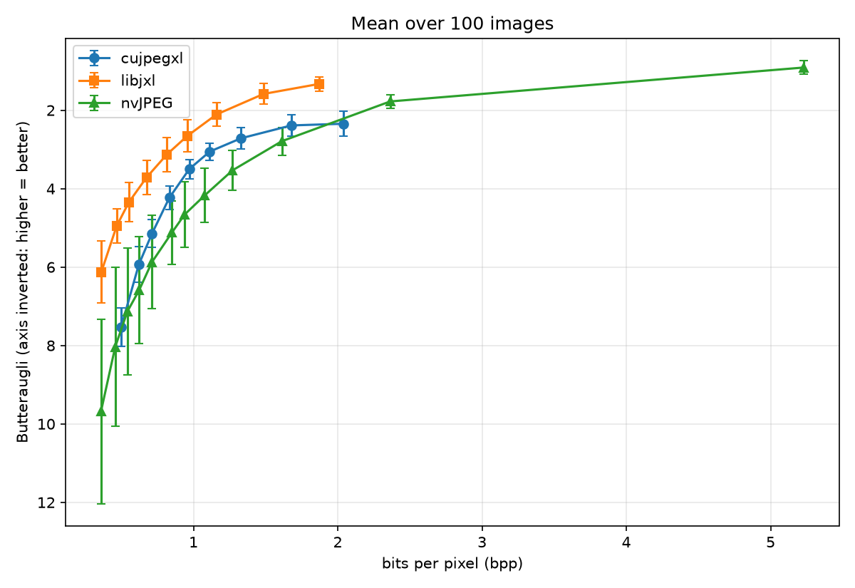
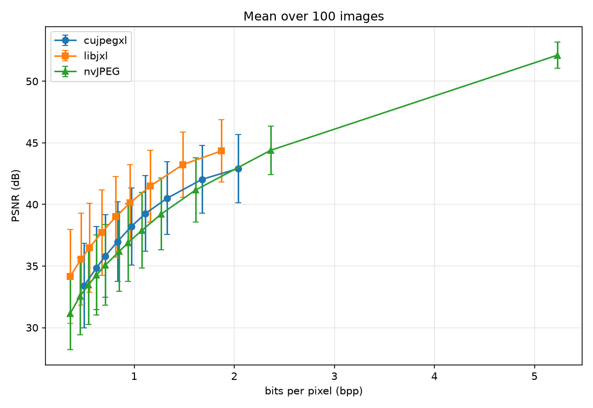
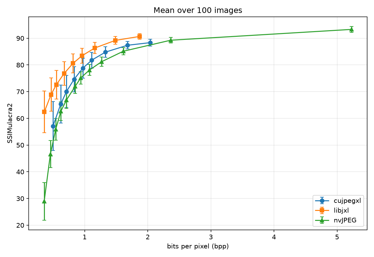 cujpegxl and libjxl sweep over target Butteraugli distances 0.5, 0.7, 1.0, 1.3, 1.6, 2.0, 2.5, 3.0, 4.0. nvJPEG sweeps over quality levels 20, 30, 40, 50, 60, 70, 75, 80, 85, 90, 95, 100.
While all three metrics agree that in general libjxl > cujpegxl > nvJPEG, the difference in perceptual metrics bears more importance than PSNR. In simple terms, PSNR gives an idea of the total signal distortion, while perceptual metrics also account for how that distortion is allocated in ways that minimize the impact on visual quality.
Considering the following input image:

Akranes lighthouse by Diego Delso on Wikimedia Commons, CC-BY-SA 4.0.
At high quality settings (distance 0.7, quality 90)15 there are limited perceivable differences. Especially at full resolution, it is hard to notice substantial visual differences, what sets the algorithms apart is especially the achieved bits-per-pixel level of compression.
Top to bottom: nvJPEG (quality 90, 2.35 bpp), cujpegxl (distance 0.7, 2.04 bpp), libjxl (distance 0.7, 2.00 bpp).
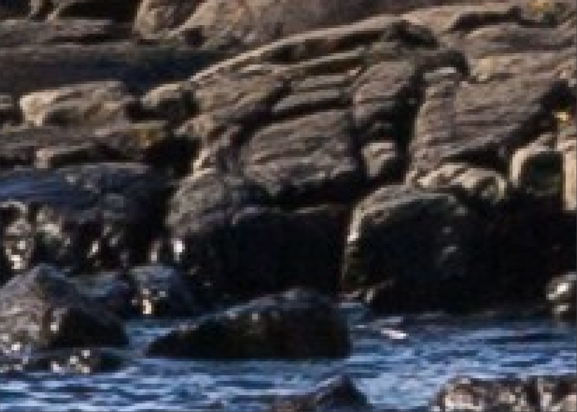
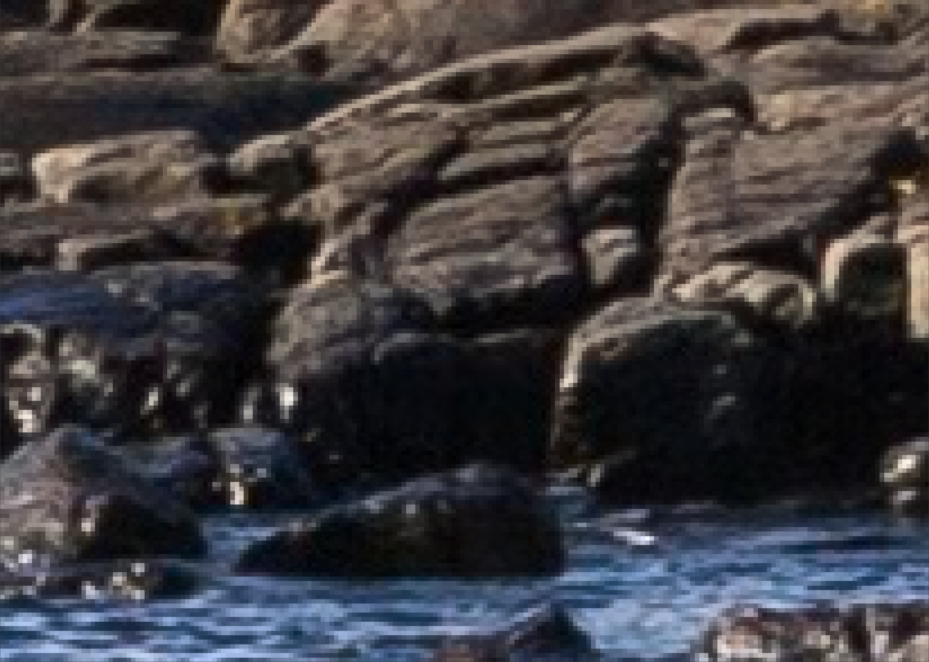
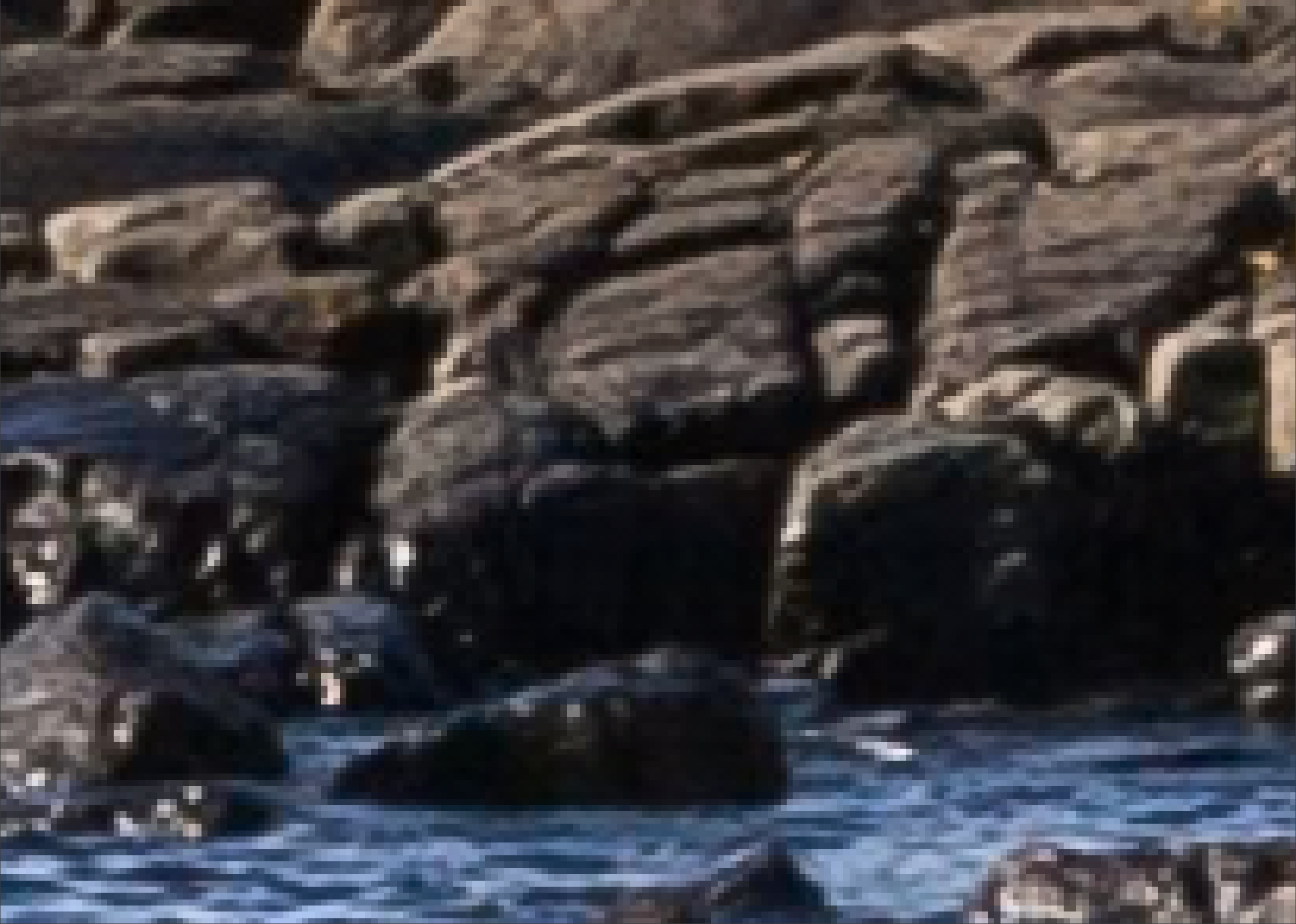
Detail of Akranes lighthouse (by Diego Delso on Wikimedia Commons, CC-BY-SA 4.0).
The difference in quality becomes more noticeable with higher compression settings. Looking at the same example (distance 3.0, quality 40), JPEG shows more noticeable artifacts, and in particular it is possible to clearly see the 8x8 DCT grid. The result from cujpegxl, at roughly the same compression rate, has substantially higher visual quality and it is noticeably less distorted. The output from libjxl looks even better and at the same time it achieves a higher compression rate.
Top to bottom: nvJPEG (quality 40, 0.88 bpp), cujpegxl (distance 3.0, 0.86 bpp), libjxl (distance 3.0, 0.65 bpp).
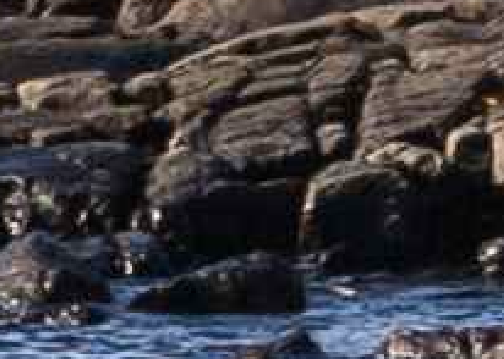
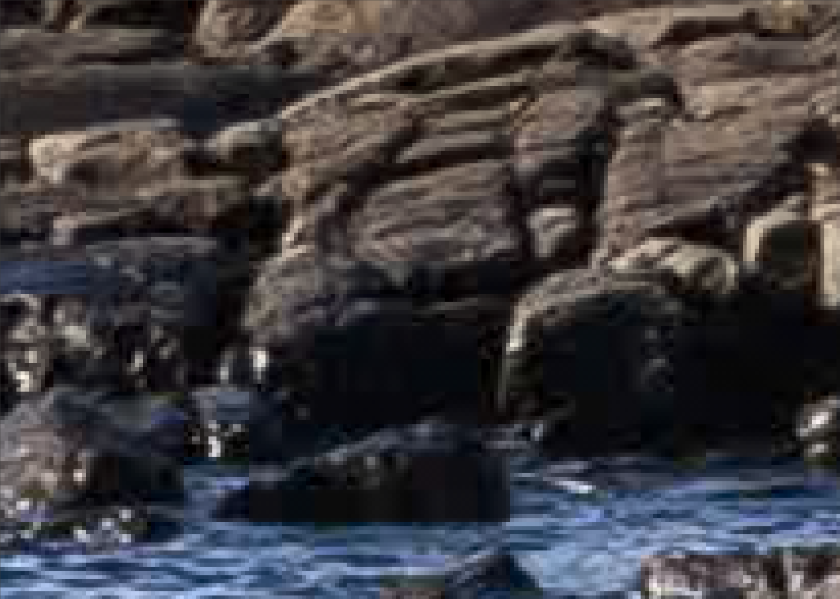
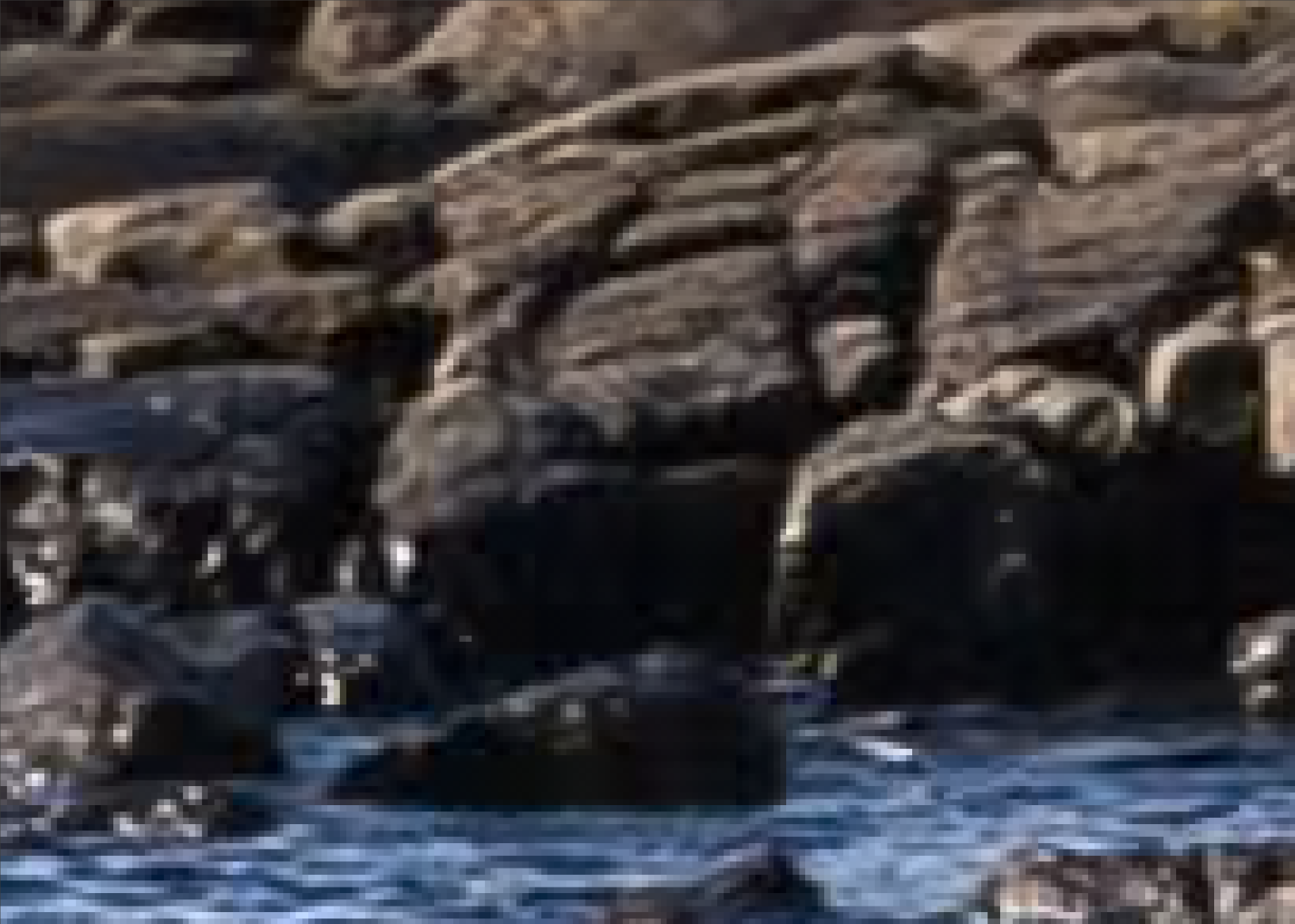
Detail of Akranes lighthouse (by Diego Delso on Wikimedia Commons, CC-BY-SA 4.0).
Performance
The encoder meets my initial requirement of >15 fps @ 4K (I measured ~21 fps on a 1080Ti), but it is still behind my final goal of sustained 15 fps on a constrained device, using maybe 5 to 10 times less resources than the current version. I think this goal should be achievable but it will require more effort and iterations.
Towards the end of this first implementation phase, the LLMs had difficulty discovering more optimization opportunities on their own (and made many inconclusive or counterproductive attempts), but I think it should be possible to work on the code structure to better exploit parallelism.16 There are also some platform-specific optimizations, such as using tensor cores and FP16 arithmetic,17 that were not supported on the GPU I used for initial development, but I would like to add later and that would yield significant improvements on newer platforms.
Another important issue was the lack of ncu support on the development GPU, meaning the AI agents were limited to custom instrumentation instead of e.g. being able to use NVTX. Giving them access to a development platform with finer-grained and more detailed microprofiling would help them in their autonomous optimization discovery.
Conclusions
This has been an interesting project, on a problem that is complex enough to still be challenging at this scale, yielding good results. It has however hit some limitations, and I am planning to further iterate on it later on to achieve even better results. I think an AI system with a larger budget (thousands of USD in usage credits) could probably chew through it with more satisfactory results and in a much more autonomous fashion, working at a smaller and cheaper scale requires instead to be smarter and more focused.
As a future direction, it will be interesting to look into an efficient GPU implementation of rANS (which is probably the biggest remaining source of lossless compression rate improvement), a broader range of VarDCT sizes and shapes, and cost-driven group clustering. Quality at a fixed compression can also probably be increased with better quantization calibration and better chroma-from-luma estimation.
The implementation is freely available on GitHub. Enjoy!
References
- J. Alakuijala, J. Sneyers, L. Versari, and J. Wassenberg, “JPEG White Paper: JPEG XL Image Coding System,” 2023.

Footnotes
-
Interestingly, modular mode can also take as input the coefficients of a JPEG-encoded image. This makes it possible to use JPEG XL to perform an additional lossless compression on top of an already (lossy) compressed JPEG image. ↩
-
The decoder generally applies a Gaborish transform (a small symmetric 3x3 convolution) to smoothen out compression artifacts. Pre-sharpening the input with an inverse Gaborish transform cancels out the loss due to the Gaborish in the decoder. ↩
-
That the encoder can estimate, usually with a mix of global and local information. ↩
-
A default perceptually-tuned weight matrix is defined, but the encoder could customize it. ↩
-
In an analogy with direct and alternating current in electrodynamics, the zero-order coefficient is called “DC” and the higher-order ones are called “AC”. ↩
-
Hilariously, sometimes agents would comment with “the complexity is immense” when picking up some implementation tasks. ↩
-
I chose the name because it is recognisable while at the same time it is unlikely to be ambiguous with built-in skills from various AI vendors. ↩
-
It should be noted, however, that I have not been reviewing the output line-by-line (as in a regular code review). I only reviewed high-level structure, design, and results, and used more AI agents to do in-detail code review. This allowed the project to move much faster. ↩
-
It would be possible to let the AI work more autonomously and have it self-decide via trial-and-error and by letting it experiment a lot more. I believe that approach would lead to potentially better results and would require less supervision, but it would also require orders of magnitude more tokens of model inference. ↩
-
JPEG XL supports \(2 \le s \le 256\). ↩
-
I have quite some experience dealing with AI optimization of high-performance code, so I am generally aware of its limitations. ↩
-
Which is unsurprising, as entropy coding is not a particularly GPU-friendly algorithm. ↩
-
It is a small set, but that is intentional to capture enough diversity while allowing for fast iteration. This set is used only for development purposes, not for evaluation nor to make any statistical conclusions. ↩
-
Note that there is no direct meaningful mapping between the JPEG 0-100 quality knob and the JPEG XL target Butteraugli distance. In these showcased examples I picked pairs of settings to compare visual quality at a roughly equivalent compression rate. ↩
-
Given the size and complexity of the project, and its very fast pace, I did not have time to look at all the code in great detail, and I could use some time to analyze the code structure more in depth to be able to provide the AI agents with more specific instructions and guidance. ↩
-
On a Pascal GPU like the GTX 1080Ti, FP16 arithmetic is several times slower than FP32, while on more recent architectures it has roughly twice the throughput of FP32. ↩