In Uppsala I spent several months investigating the generation of displacement fields with known volume changes, and I even implemented a software suite for the purpose. This might seem an odd topic to pick as working subject, so it is worth a bit of clarification about its purpose and applications.

My voyage in the realm of displacements with known volume changes stems from the work on image registration I did at Akademiska sjukhuset, the Uppsala University Hospital, around the time I was working on my master’s thesis in computer science. I think this is an interesting topic of research, and this post aims to explain what it is and how it relates with displacement fields and Jacobian determinants.

Imiomics in a nutshell

Imaging-omics, or imiomics for short, is a medical image analysis methodology introduced at Uppsala University in 2017, that allows to study and visualise pointwise correlations between the local body composition and non-image biomarkers [1]. In this context, “body composition” denotes local information such as the volume and composition of tissues in each point of the body, while non-image biomarkers can be for instance body measurements (height, weight, waist circumference, etc.), blood analysis values, physical test (bioimpedance, VO₂ max, etc.), and any other numeric measures that can be associated to a subject.

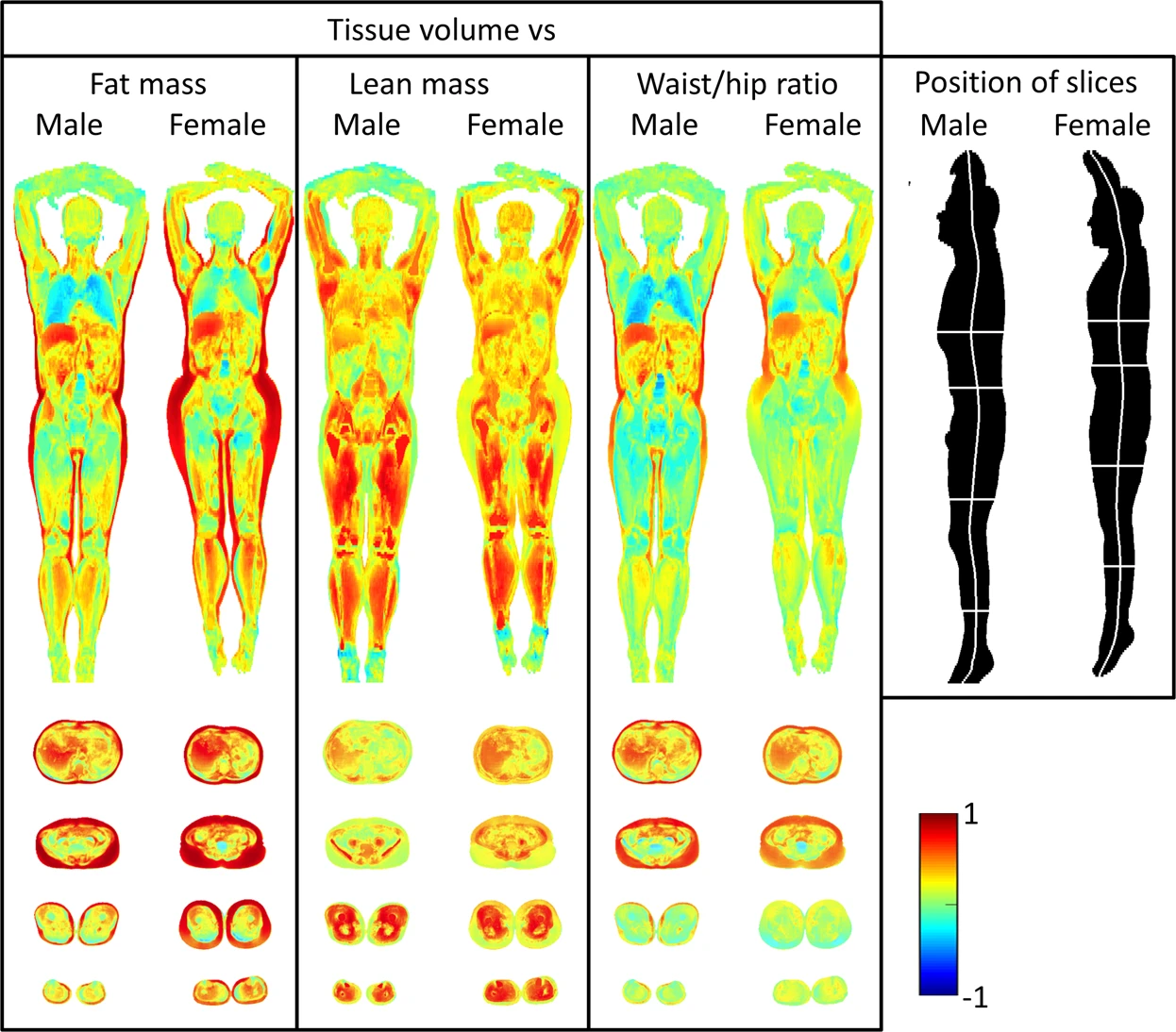
In other words, imiomics makes it possible to visualise a correlation map between some local physical property of the body and other global measures. The following example from Lind et al. [2] gives a clear idea of the power of such approach, showing the correlation between adipose tissue volume and total fat mass, lean mass, and waist-hip ratio. Clear correlations are visible, such as a positive one between subcutaneous tissues in the hips and total fat mass, and a negative one between lung volume and total fat mass:

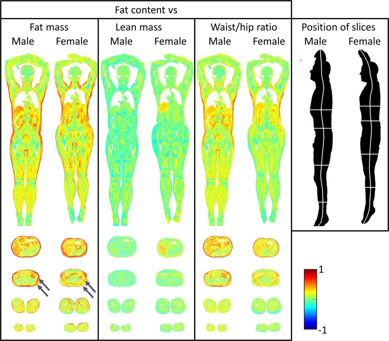
While probably such results do not come as a surprise, they prove the concept to be working and demonstrate the potential of such technique, that can be used to discover and study less obvious correlations and produce novel results. Another example from the same paper shows the correlation between the local fat content and the same scalars as in the previous example. This time it shows a different and probably less intuitive picture, with high fat mass strongly correlated with the fat content in a much thinner layer of subcutaneous fat:

In addition to the group studies in the example above, imiomics is suitable for other types of statistical analysis, such as longitudinal studies, where the evolution of a single subject is followed up through time, or anomaly detection, where discrepancies between a subject and a normality atlas (e.g. the presence of lesions) are identified [3].

Technicalities under the hood

The local fat and water content can be easily measured with a non-invasive and radiation-free approach, by using fat-water separated magnetic resonance imaging (MRI), making it ideal for investigation studies. The addition of positron emission tomography (PET) data, that gives a functional insight of the metabolic processes, allows broader applications to fields such as oncology. These are well known imaging techniques that have been around for decades, but the innovative part of imiomics is how they are exploited to make it possible to preform group studies at voxel resolution.

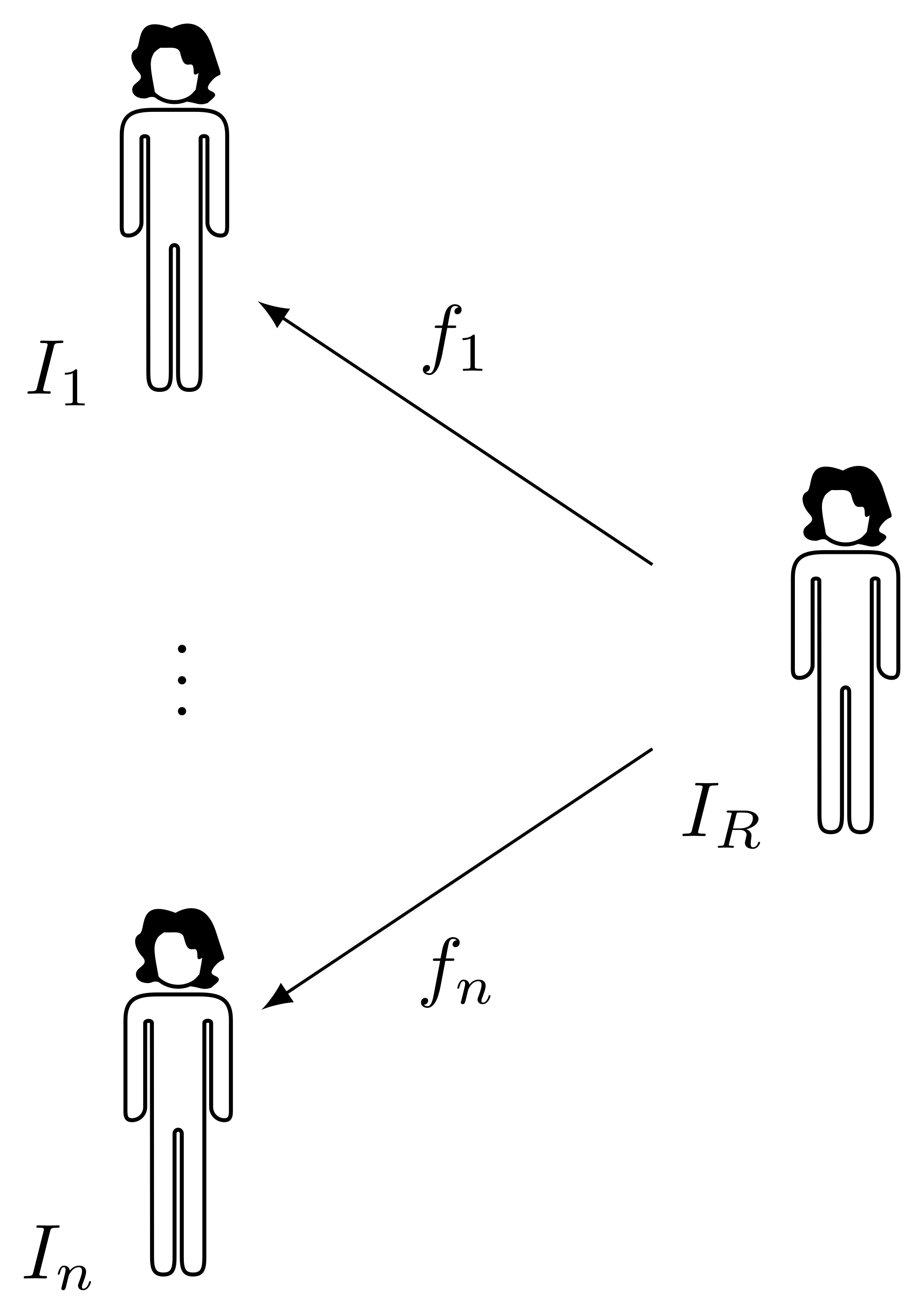
Given a cohort composed by \(n\) subjects \(I_1, \dots, I_n\), the key idea is to construct an atlas \(I_R\) representative of the group, and to register all subjects to it. Whole body registration is a difficult task, due to high intra-subject anatomical and pose variability. A deformable registration method based on graph cut optimisation allows to get a pointwise transform with sub-voxel accuracy, robustly handling difficult cases and with fast computational time [4]. If PET data is collected together with the MR data by using a combined scanner, therefore producing inherently co-registered PET and MR images, the transform obtained by registering the MR can be used to also warp the PET data, allowing to produce a PET atlas.

After all subjects are registered to the common reference space, each voxel of the atlas is mapped to a point in each subject \(I_k\) by a transform \(f_k\), forming a vector of samples that can be used for statistical analysis.¹ Moreover, the spatial Jacobian determinant \(J[f]\) of a transform \(f\) mapping the atlas to subject \(I_n\)

gives the local volume change induced by \(f\) at point \(\boldsymbol{x}\), that represents the local tissue volume of subject \(I_n\) at point \(\boldsymbol{x}\) with respect to the reference space. A Jacobian determinant equal to one denotes no volume change, a value greater than one denotes local expansion, a value between zero and one denotes local compression. Values lesser or equal than zero denote a physically unfeasible transform, and typically emerge from errors or imperfections in the image registration process.²

While the transform \(f\) maps points from reference space coordinates to source image coordinates, in the context of image registration it is often convenient to express the deformation as a displacement \(d\), i.e. the difference between the transform \(f\) and the identity, that tells how much a point needs to be displaced from its reference space coordinates in order to reach its position in source image coordinates.

From this it naturally follows that the Jacobian determinant of a transform equals the determinant of the Jacobian matrix of its associated displacement summed with the identity matrix

where \(\delta_{ij}\) is Kronecker’s delta function. This is a small and simple detail, but it can nevertheless be a source of confusion. In the following, the Jacobian determinant is always the Jacobian of the transform, not the one of the displacement, since the latter does not express the local volume change induced by the transform.

Reference space

Given a good dataset and a robust registration method, the only remaining issue is how to determine the atlas to be used in the registration process. The problem of determining an optimal and unbiased atlas for the registration of a population has been an intense topic of study, especially in the field of neuroimaging, leading to the development of what is known as groupwise image registration. While classical image registration solves the problem of finding a common coordinate system for a pair of images, and it can be applied iteratively, one pair of images at time, to register a population to a common frame, groupwise registration aims to register an entire group of images to a frame that is optimal for the population as a whole.

Several groupwise registration methodologies have been developed since the early 2000s, including pairwise registration to an explicit template that is iteratively warped according to some average property of the individual transforms [5], [6] and implicit methods that construct the set of transforms for all images simultaneously, optimising some groupwise metric defined over all images and transforms [7], [8]. Interestingly, the latter approach does not require any choice of template image a priori, and it does not produce any explicit reference image but only a set of transforms. If desired, a reference image can be recovered by averaging the warped subjects.

While groupwise methods, especially implicit methods, nicely address the problem of the bias toward an arbitrary reference space in the registration of a populations, often with elegant theoretical frameworks, in practice they still present some inconveniences. Groupwise approaches can have difficulties to handle large deformations and finely align structures, and this represents an issue, since imiomics requires a fairly accurate registration. Moreover, the computational cost and memory footprint of implicit methods increase with the size of the group being registered: if the groupwise transform has the form of \(T(\boldsymbol{\mu})\), where \(\boldsymbol{\mu}\) is the vector of all parameters from all transforms, and the groupwise metric is defined over the \(n+1\)-dimensional volume obtained by stacking the input images \(I_1, \dots, I_n\), the cost of optimisation is going to grow (super-linearly, in most cases) as a function of the population size. This makes it difficult to scale to large populations, especially when considering the size of whole body images, typically larger than the brain images used in the development of most groupwise methods.

Optimising the reference space

Given the practical limitations of implicit groupwise methods, registration of the population can be done in a pairwise fashion against an explicit reference image. A good reference can be a subject from the cohort with “average” properties, such as size and weight, that is representative of the normal anatomy of the cohort, and possibly having good quality of image acquisition (such as the absence of imaging artefacts). Moreover, given the importance of tissue volume in many imiomics applications, a desired property of the reference space is what we can call “neutrality with respect to volume changes”: when mapping the reference to all subjects, the average volume change in each point of the reference space should be null. Since we measure volume change through the Jacobian determinant of the transforms, and a unit Jacobian implies conservation of local volume, the geometric mean of the Jacobian maps for all subjects should be one in all points of the reference space.

While it is usually possible to reasonably fulfill the first property of good representativity of the cohort, by carefully selecting a reference, the last requirement on neutrality with respect to volume changes is unlikely to happen by chance. Since the subcutaneous fat deposits contribute to a significant portion of the body volume variability for subjects of comparable height, a possible heuristic is to select as the reference a subject that both height and total fat mass³ simultaneously close to the respective medians for the population. This helps to get a good guess of the average volume for the cohort, but it is obviously far from having the desired mean volume everywhere in a pointwise fashion [9].

In principle, this issue could be overcome in different ways. One possibility would be to perform an implicit-reference groupwise registration, adding a regularisation term to penalise a mean Jacobian far from one. While this appears to be an elegant solution, there are practical concerns that make it hard to apply. One is the computational cost of groupwise registration, both in terms of memory footprint and time complexity, that grows (often superlinearly) with the size of the cohort of subjects, making it unfeasible to register large populations. Another concern is the intrinsic difficulty of whole body registration, that requires robust deformable registration methods in order to obtain transforms sufficiently accurate for imiomics analysis.

An alternative approach, used in some early groupwise registration methods [5], [6], is to start with a subject from the cohort as initial template, and iteratively refine it and repeat the registration to the refined template, until the set of transforms from the template towards the rest of the cohort satisfy a desired property. Thinking of the images as points in some feature space, the intuitive idea is to have the initial subject (red circle) iteratively moving in the feature space (red squares) and converging to the mean of the population (black circles), for some definition of mean that suits the problem.

Since the images can be registered one pair at a time, this approach has a constant memory footprint and a time complexity that is linear in the size of the cohort. Moreover, it is possible to apply any robust pairwise registration algorithm, without having to face potential convergence struggles of implicit groupwise methods in difficult scenarios.

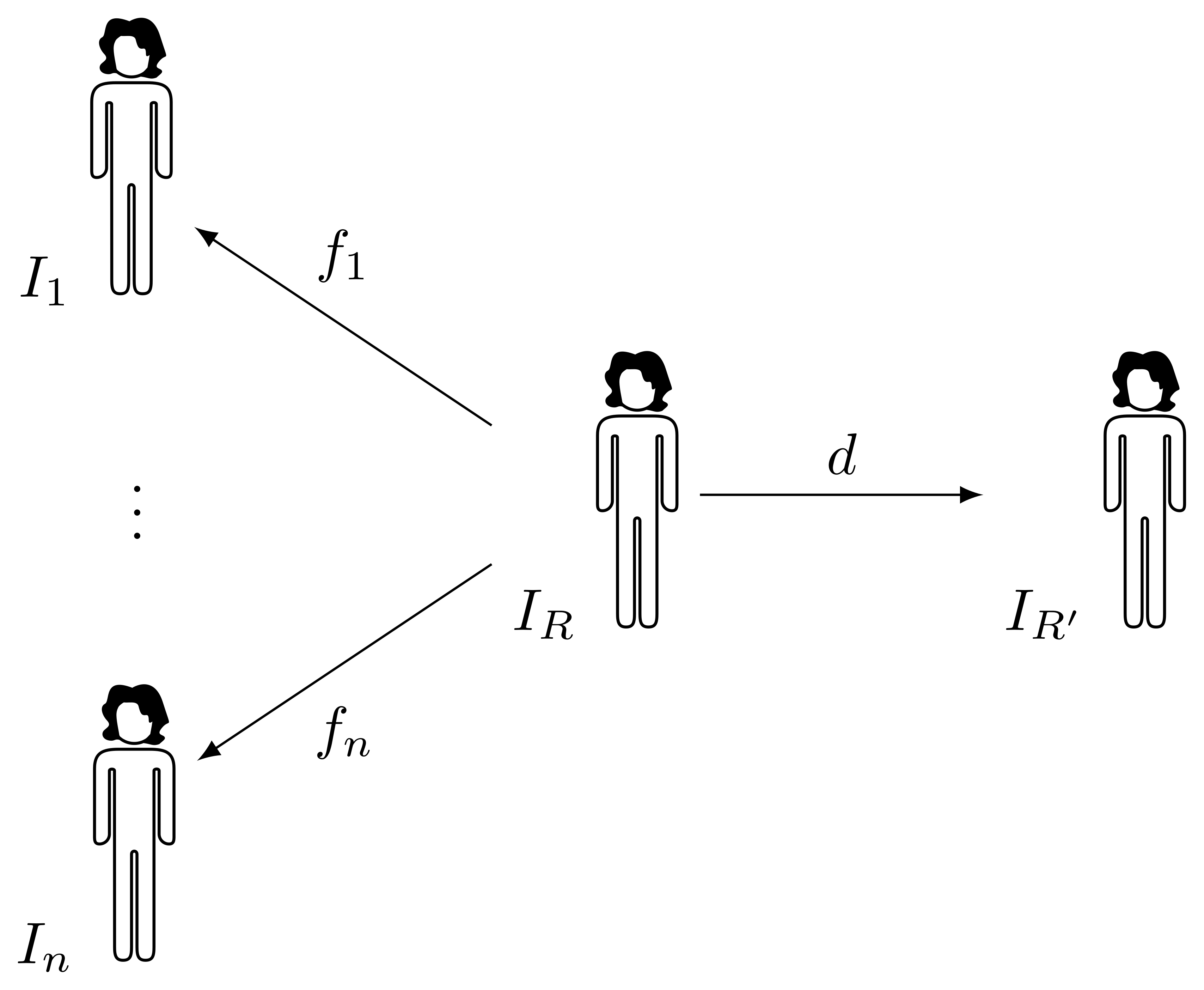
At each iteration, a registration of the images \(I_1, \dots, I_n\) in the group to the current template \(I_R\) is performed, producing a set of transforms \(f_1, \dots, f_n\) with a certain mean Jacobian \(J\), and the iterative correction \(d\) should somehow produce a new template \(I_{R'}\) such that the mean Jacobian of \(f_1 \circ d^{-1}, \dots, f_n \circ d^{-1}\) is closer to one in every point. A reasonable approach is to pick a deformation \(d\) such that its Jacobian is exactly \(J\), therefore cancelling the residual mean volume. Ideally, this could be done in a single iteration and, if everything was perfect, a new registration of all subjects to the new reference \(I_{R'}\) should produce as deformations exactly \(f_1 \circ d^{-1}, \dots, f_n \circ d^{-1}\). Alas, this is not likely to happen, due to the imperfection of the registration methods and to limitations in accuracy of numerical operations. However, it is possible to iterate rounds of registration to the new reference and generation of a new template, until convergence.

The only remaining issue is how to produce a deformation with given Jacobian determinant. Unfortunately, without further constraints, this is an ill-posed problem, since infinite transforms can share the same Jacobian determinant.

Generation of dense deformations with known volume changes

One possibility is to model the problem as a mechanical deformation. In principle, different assumptions can be made, leading to different deformation models, and the resulting system of partial differential equations can be solved numerically, for instance with finite differences [10] or finite elements [11], [12].⁴ This approach has some advantages, such as a well understood mathematical and physical model, and the possibility to control the physical properties of the tissues being deformed by manipulating the parameters of such model. On the downside, however, the numerical solution of this problem on the scale of a whole body image can be expensive in terms of memory and computing time. Moreover, finite elements require a meaningful mesh generation, that constitutes a whole problem on its own.

Another approach is constituted by search based methods. It is possible to perform a search in the space of displacements by optimising a cost function that accounts for the distance between the Jacobian determinant \(J_\boldsymbol{d}\) of the deformation associated to displacement \(\boldsymbol{d}\) and the desired Jacobian \(J^*\) [13], [14]. While this approach may look tricky in principle, due to the fact that infinite solutions exist, by using a null displacement as initial guess it is likely to end the search in a reasonably good solution.

A simple yet effective example of cost function for this problem is the squared difference

Such function is differentiable with respect to the components of the displacement, therefore it is possible to perform gradient descent to minimise it. It is also possible to add a regularisation term to penalise non-smooth and physically unfeasible deformations, if necessary [13].

Given a displacement \(d(x,y,z) = \left(f(x,y,z), g(x,y,z), h(x,y,z) \right)\), the partial derivatives in the expression of the Jacobian can be discretised with central differences of step length \((\delta_x, \delta_y, \delta_z)\), allowing to write the gradient of \(E\) in closed form. The partial derivative of \(E\) with respect to the component \(f\) of the discrete displacement at coordinates \((x, y, z)\) is given by

denoting with \(e^{x,y,z} = J_{\boldsymbol{d}}(x,y,z) - J^*(x,y,z)\) the local distance to the target Jacobian, and with \(f_x^{x,y,z}\) the central difference \(\frac{1}{\delta_x} \left(f(x+1,y,z) - f(x-1,y,z) \right)\).

This expression is a bit cumbersome, and it is possible to greatly cut the calculations by throwing away all cross terms and approximate the gradient as [14]

It is possible to experimentally observe how removing the cross terms worsens the improvement at each iteration and weakens the robustness of the search, but the savings in terms of computing time are so big that in many cases it is possible to compensate by performing more iterations and still reach a better solution within the same computing time [15].

Regardless of whether the full gradient or its approximation is used, it is possible to parallelise calculations for all voxels independently, making this algorithm suitable for OpenMP and GPU computing.

An important trick to keep in mind is to mask a region of interest in the image, and to relax the search outside it by reducing the cost of a mismatching Jacobian in the background. This allows to redistribute the residual volume change outside the body, greatly helping convergence. Otherwise, the deformation would propagate to the boundary of the image volume, and if the total volume change over the image does not integrate to zero the method would not converge to a solution at all.

Some results

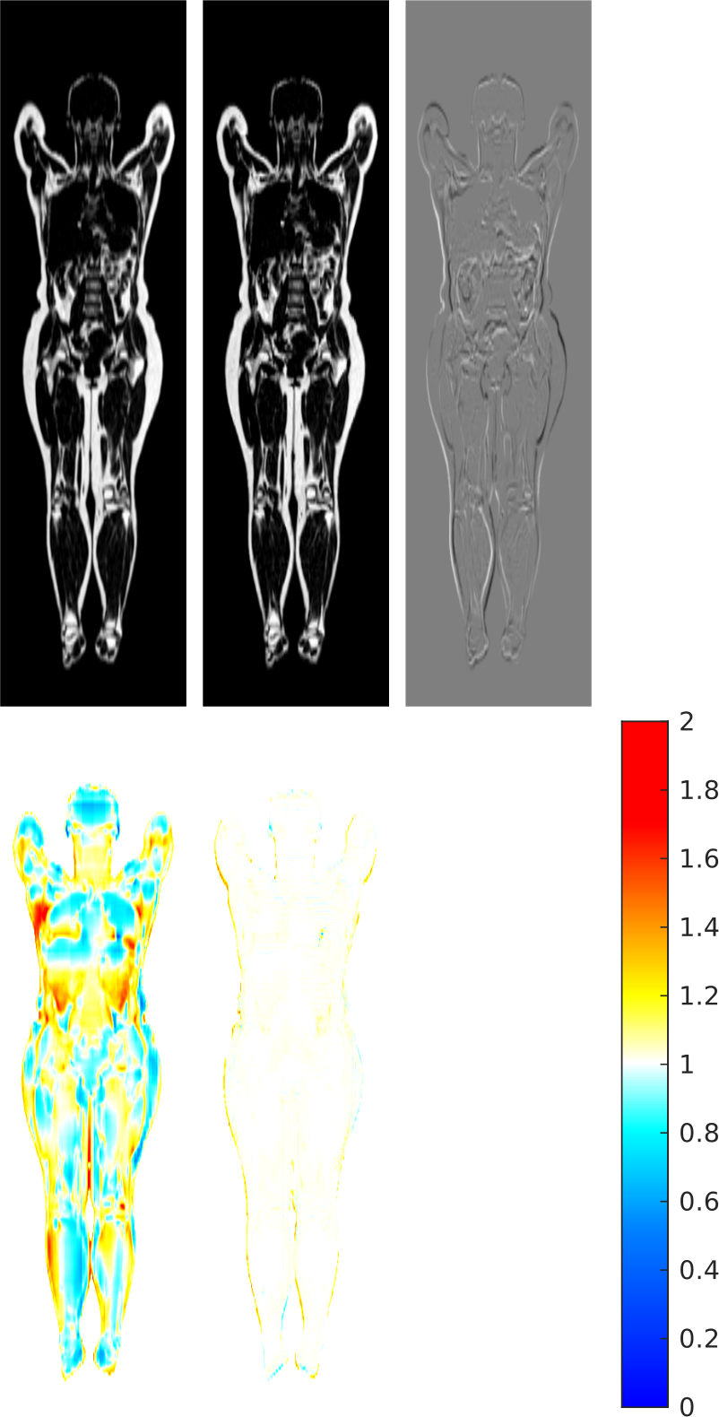
Going back to the whole body group registration problem, now we have all the tools to generate a synthetic whole body atlas with zero average volume change. Given a cohort of 167 subjects, a subject with height and fat mass close to the median is used as initial reference space (top-left panel), and the average Jacobian (bottom-left panel) of the transforms that map it to the cohort is far from being constant unitary. From this Jacobian, a displacement is generated and its inverse is used to sample a new reference space (top-centre panel). The difference image (top-right panel) shows how the anatomy is overall preserved and tissue volumes are locally adjusted. When mapping the cohort to this new reference space, this time the Jacobian (bottom-centre panel) is close to one almost everywhere [9].

It is fascinating to observe how this simple approach for the generation of a displacement with given Jacobian can be applied on a relatively complicated target. The Jacobian in this example shows a significant range of values, often with sharp transitions (made harder by the low resolution of the image) and sometimes with bad values, being close to zero in different regions (due to local imperfections in the registration process, that cause unreasonably high compression of the tissues in parts of the body). By comparison, previous applications of this technique in neuroimaging made use of piecewise constant target Jacobians, with only values of small magnitude.

Source code

A complete implementation of the two methods, running both on CPU (implemented in C) and GPU (implemented in CUDA), with convenient Python wrappings, is available on GitHub and PyPI as the disptools package. Enjoy!

References

1. R. Strand et al., “A concept for holistic whole body MRI data analysis, Imiomics,” PloS one, vol. 12, no. 2, 2017.
2. L. Lind, J. Kullberg, H. Ahlström, K. Michaëlsson, and R. Strand, “Proof of principle study of a detailed whole-body image analysis technique, ‘Imiomics’, regarding adipose and lean tissue distribution,” Scientific reports, vol. 9, no. 1, p. 7388, 2019.
3. T. Sjöholm et al., “A whole-body FDG PET/MR atlas for multiparametric voxel-based analysis,” Scientific reports, vol. 9, no. 1, p. 6158, 2019.
4. S. Ekström, F. Malmberg, H. Ahlström, J. Kullberg, and R. Strand, “Fast graph-cut based optimization for practical dense deformable registration of volume images,” Computerized Medical Imaging and Graphics, vol. 84, p. 101745, 2020.
5. A. Guimond, J. Meunier, and J.-P. Thirion, “Average brain models: A convergence study,” Computer vision and image understanding, vol. 77, no. 2, pp. 192–210, 2000.
6. G. Wu, H. Jia, Q. Wang, and D. Shen, “SharpMean: groupwise registration guided by sharp mean image and tree-based registration,” NeuroImage, vol. 56, no. 4, pp. 1968–1981, 2011.
7. S. K. Balci, P. Golland, M. Shenton, and W. M. Wells, “Free-Form B-spline Deformation Model for Groupwise Registration,” in MICCAI. International Conference on Medical Image Computing and Computer-Assisted Intervention, 2006, vol. 10, pp. 23–30.
8. S. Joshi, B. Davis, M. Jomier, and G. Gerig, “Unbiased diffeomorphic atlas construction for computational anatomy,” NeuroImage, vol. 23, pp. S151–S160, 2004.
9. M. Pilia, J. Kullberg, H. Ahlström, F. Malmberg, S. Ekström, and R. Strand, “Average volume reference space for large scale registration of whole-body magnetic resonance images,” PLOS ONE, vol. 14, no. 10, pp. 1–15, 2019.
10. B. Khanal, N. Ayache, and X. Pennec, “Simulating Longitudinal Brain MRIs with known Volume Changes and Realistic Variations in Image Intensity,” Frontiers in Neuroscience, vol. 11, no. Article 132, p. 18, 2017.
11. A. D. C. Smith, W. R. Crum, D. L. Hill, N. A. Thacker, and P. A. Bromiley, “Biomechanical simulation of atrophy in MR images,” in Proceedings of SPIE, 2003, vol. 5032, pp. 481–490.
12. O. Camara et al., “Phenomenological model of diffuse global and regional atrophy using finite-element methods,” IEEE transactions on medical imaging, vol. 25, no. 11, pp. 1417–1430, 2006.
13. B. Karaçali and C. Davatzikos, “Simulation of tissue atrophy using a topology preserving transformation model,” IEEE transactions on medical imaging, vol. 25, no. 5, pp. 649–652, 2006.
14. M. C. van Eede, J. Scholz, M. M. Chakravarty, R. M. Henkelman, and J. P. Lerch, “Mapping registration sensitivity in MR mouse brain images,” Neuroimage, vol. 82, pp. 226–236, 2013.
15. M. Pilia, “Groupwise whole-body MR image registration guided by zero-average volume changes,” Master's thesis, Acta Universitatis Upsaliensis, 2018.

Footnotes