Currently, I work mostly on image registration algorithms, and I devoted quite some time looking into groupwise registration techniques. In its essence, groupwise registration is a process that aligns multiple images, mapping them to a common reference space, without having to explicitly define such reference space (e.g. without manually selecting one image as the reference).

I work with problems that involve large deformations and great anatomical variability, making it difficult to achieve robust automatic registration. In some pairwise registration tasks, landmark-based registration has proven to be useful, especially to initially guide the transform, giving a better initial estimation that improves the robustness or the process. For this reason, I decided to look for a similar approach in a groupwise setting.

\(\newcommand{\bmu}{\boldsymbol{\mu}} \newcommand{\bx}{\boldsymbol{x}} \newcommand{\obx}{\bar{\bx}} \newcommand{\fpart}[2]{\frac{\partial {#1}}{\partial {#2}}}\)

Groupwise registration in a nutshell

There are different approaches to groupwise registration, and the most popular ones involve the use of an implicit reference space, without using any explicitly selected template. Such space is implicitly defined by a collection of transforms that map from reference space to the moving images, and that are are optimised simultaneously.

Having one transform for each moving image implies that the size of the search space grows at least linearly with the number of moving images registered together. This has a cost in terms of memory and computing time that, especially when working with volume images, can soon become prohibitive. For this reason, parametric models and subsampling techniques are often employed in this context.

The target of the optimisation is a similarity function defined over the whole set of images: one of the simplest, that works well for normalised images that share the same distribution of intensities, is is the standard deviation of the intensity of all the points in the moving images mapped from a certain position in reference space [1], which can be considered the groupwise equivalent of mean squared difference similarity in classical pairwise registration. This is a suitable choice, for instance, when dealing with imaging modalities such as cardiac cine MR. In other settings, such as diffusion imaging, contrast varies over time and the assumption of similar distribution of intensities does not hold anymore, hence more sophisticated techniques are required to separate the intensity dissimilarity due to changes in contrast from the dissimilarity due to misalignment (e.g. metrics based on principal component analysis [2].

Groupwise registration with Elastix

While I work most of the time with non-parametric deformation models, sometimes I also rely on Elastix [3], a deformable registration toolbox for medical image processing that offers a variety of parametric transform models and several image similarity metrics. Its workhorse is the B-spline transform, which can be paired with rigid or affine pre-registration and can combine multiple images and multiple metrics (among the various that are implemented) in a single registration process, including a CorrespondingPointsEuclideanDistanceMetric for pairwise landmark-based registration. All of this is made possible in practice thanks to an implementation of stochastic gradient descent (SGD) with adaptive parameters [4], which makes it possible to robustly optimise the energy for this problem within an acceptable computing time.

While most Elastix features are designed for pairwise registration, the toolbox also offers some support for groupwise registration. The trick used to fit groupwise registration within the pre-existing software framework is to represent a group of n-dimensional images as a n+1-dimensional volume, e.g. a 4D image for a group of 3D volumes, where the first three indices are spatial coordinates within each volume, and the last index identifies the single volumes within the group. This choice is actually very reasonable, given that often groupwise registration is used to align the frames of a time series, which is inherently n+1-dimensional. To simplify the description, in the following I will refer to such additional axis as the last dimension or the time axis (even when the volume does not represent a time series).

With this setup, it is possible to have a metric that uses only the moving image, which will be the n+1-dimensional volume representing the group of images, and to use a transform that maps from an implicit reference space to such volume. However, just using a regular n+1-dimensional transform is unlikely to give the expected results, since we do not want to allow movements along the last dimension, i.e. between different images.¹ For this reason, a special BSplineStackTransform is implemented for groupwise registration: as the name suggests, it is actually a set of stacked n-dimensional transforms, each of whom is applied independently to a single slice along the time axis.

Making the landmarks groupwise

Elastix does not natively offer groupwise landmark-based registration, so I decided to implement a metric component myself to try this approach. While in literature there are several interesting works on unlabeled point set registration methods [5], [6], in this scenario the task is a bit easier, since the correspondence between landmarks is already known. In the pairwise case it is straightforward to define a dissimilarity with energy \(E\) for the correspondence, e.g. by minimising the mean Euclidean distance between pairs \((\bx^f_i, \bx^m_i)\) of corresponding points in the fixed and moving image

where \(\bmu\) is the vector of parameters for the transform \(T\) that maps points from the reference space (in the fixed image) to the moving image.

The groupwise scenario is more complicated due to the fact that there is no known position in reference space, all we know is the position of each occurrence of the \(m\) landmarks in the \(n\) moving images. Since we want all the transforms to map the same point in reference space to all the occurrences of a landmark in the moving images, an ideal and unbiased approach could be to minimise, for each landmark \(\bx^i\), the variance of the preimages of all its occurrences \(\bx^i_j\) in the moving images.

Unfortunately, in practice this is not immediate to do in Elastix, since we do not know the inverse \(T^{-1}\) of the transform and, for all we know, it may not even be invertible in general (e.g. when using B-splines).

For this reason, I tried an alternative approach, approximating the mean of the preimages with a central tendency estimator of the landmarks themselves, and then moving the optimisation to the moving image space.

This is of course a bold approximation that somehow introduces a bias in the construction of the reference space, but if the choice of the landmarks is reasonable and their position is reliable, it may still lead to some useful results. For simplicity I am using the mean of the landmarks, but other estimators more robust with respect to outliers, such as the median, can be used in principle, since at this point we do not require the estimator itself to be differentiable. To make things a little simpler in practice we can consider a different energy function that shares the same optima:

whose derivative with respect to the parameters of the transform is

where \(\obx^i\) is the mean position of the i-th landmark

Implementing the metric

Now that we have an expression for the energy and its derivative, all that is left to do is to write an Elastix component that implements it. A good starting point is to have a look at the implementation of the CorrespondingPointsEuclideanDistanceMetric. Elastix metrics implement the main logic within a class in the itk namespace, and the registration-related logic in a subclass of the latter, in the elastix namespace, so for example we see the itk::CorrespondingPointsEuclideanDistancePointMetric class, that inherits from itk::SingleValuedPointSetToPointSetMetric and that is inherited by elastix::CorrespondingPointsEuclideanDistanceMetric.

A simple solution is to use the same approach for our new metric. The obvious drawback is that, being a subclass of itk::SingleValuedPointSetToPointSetMetric, it will require two point set input files, one for the fixed and one for the moving points. The solution is to leave things as they are, and just pass a dummy file for the fixed points when calling Elastix, whose content will simply be ignored. This same approach is already used in the implementation of the groupwise registration image metrics, that require to pass a dummy fixed image as input.

Concerning the point file, it will be necessary to impose a precise order of the points to be able to group the occurrences of each landmark correctly. A possible solution is to sort all points by image, i.e. having all the landmarks of the first image together, followed by the landmarks of the second image, and so on, and imposing the same order of the landmarks across different images. The order of the images is given by their index in the time axis. This way, if we have \(m\) landmarks and \(n\) images, the file will contain \(m \cdot n\) points, and the point in position \(k\) in the file will be the occurrence of landmark \(k \mod m\) in the image \(k \div n\) (if we count starting from zero, and denote with \(\div\) the integer division operator).

x00 y00 z00 0  // image 0, landmark 0
x01 y01 z01 0  // image 0, landmark 1
     ...
x0n y0n z0n 0  // image 0, landmark n

x10 y10 z10 1  // image 1, landmark 0
x11 y11 z11 1  // image 1, landmark 1
     ...
x1n y1n z1n 1  // image 1, landmark n

  .........

xm0 ym0 zm0 m  // image m, landmark 0
xm1 ym1 zm1 m  // image m, landmark 1
    ...
xmn ymn zmn m  // image m, landmark n

The first thing to do will be to compute the mean position of each landmark once, which can be done in the Initialize() function of the CorrespondingPointsMeanDistancePointMetric class, since its value will be constant through the optimisation process.

// Group the occurrences of all landmarks in a data structure
// ...

/** Compute the mean for the occurrences of each landmark */
for( auto & landmark : m_Landmarks )
{
  landmark.mean.Fill( NumericTraits< MovingPointValueType >::ZeroValue() );
  for( const auto & p : landmark.occurrences )
  {
    landmark.mean.GetVnlVector() += p.GetVnlVector();
  }
  landmark.mean.GetVnlVector() /= landmark.occurrences.size();
}

Here we follow the code style conventions of ITK and Elastix, with two spaces indentation, opening curly braces in a new line, and spaces inside all types of parentheses. It may seem a minor point, but this style actually helps making the code more readable, since ITK programs tends to have dense and verbose sources.

The metric and its derivative will be computed together in the GetValueAndDerivative function, and separately in the GetValue and GetDerivative function. Since this metric is relatively cheap to evaluate, I avoid duplication by using the first function within the implementation of the other two, but it would make sense to have a separate, optimised implementation at least for GetValue. On the other hand, since computing the value has a negligible cost when the derivative is also computed together, it makes sense to simply call GetValueAndDerivative in the implementation of GetDerivative.

Since the energy is expressed as a sum over the points, all of whom provide an independent contribution, the key part will naturally be a loop over all the points.

PointIterator pointItMoving = movingPointSet->GetPoints()->Begin();
PointIterator pointEnd      = movingPointSet->GetPoints()->End();
int point_no = 0; // position of the current point in the list
while( pointItMoving != pointEnd )
{
  // do something with the point ...

  ++pointItMoving;
  ++point_no;
}

The base class has a m_Transform member that, unsurprisingly, represents the current transform. In order for this to make sense, we will assume it to be a BSplineStackTransform. We can compute the image of a point through the transform with its member function TransformPoint()

mappedPoint = this->m_Transform->TransformPoint( meanPoint );

Since Elastix supports the use of image masks to focus the registration within a region of interest (ROI), we make sure that the image of the mean point we are considering falls within the mask

if( this->m_MovingImageMask.IsNotNull()
    && ! this->m_MovingImageMask->IsInside( mappedPoint ) )
{
  // skip the point
}

The transform also exposes a Jacobian() member function to get the derivative of the transform with respect to its parameters, which is referred as the Jacobian.² The Jacobian is returned in a sparse representation formed by the matrix columns containing any non-zero entry, together with another vector containing the indices of the parameters that have non-zero Jacobian. This is motivated by the fact that B-splines have local support, so for a given point we expect most of the entries in the Jacobian matrix to be zero.

this->m_Transform->GetJacobian( meanPoint, jacobian, nzji );

After computing the image of the mean point in moving space and the relative Jacobian, we have all the information needed to compute the contribution of the point to the metric and its derivative. The following code snippet is in fact very close to what is done in the itk::CorrespondingPointsEuclideanDistancePointMetric class, that is built-in in Elastix.

/** Update the mean */
VnlVectorType diffPoint = ( movingPoint - mappedPoint ).GetVnlVector();
diffPoint[ m_LastDimension ] = 0.0;
MeasureType distance = diffPoint.magnitude();
measure += distance;

/** Calculate the contributions to the derivatives with respect to each parameter. */
if( distance > vcl_numeric_limits< MeasureType >::epsilon() )
{
  VnlVectorType diff_2 = diffPoint / distance;
  if( nzji.size() == this->GetNumberOfParameters() )
  {
    /** Loop over all Jacobians. */
    derivative -= diff_2 * jacobian;
  }
  else
  {
    /** Only pick the nonzero Jacobians. */
    for( unsigned int i = 0; i < nzji.size(); ++i )
    {
      const unsigned int index  = nzji[ i ];
      VnlVectorType      column = jacobian.get_column( i );
      derivative[ index ] -= dot_product( diff_2, column );
    }
  }
} // end if distance != 0

Example

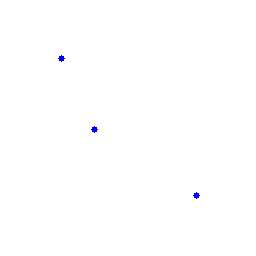
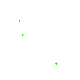
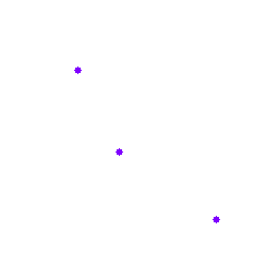
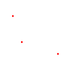
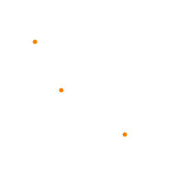
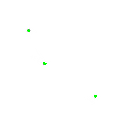
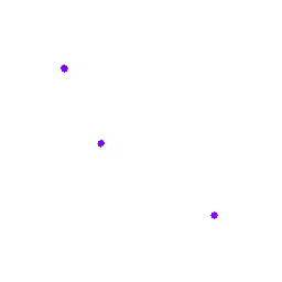
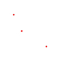
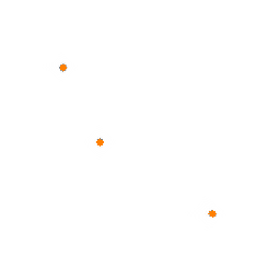
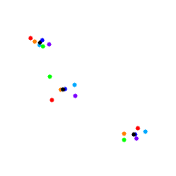
To test the metric, we generate a set of simple images. Each image contains three circles, and we put a landmark in the centre of each circle. We use a different colour for each image to make it easier to visualise.

import cv2
import numpy as np

np.random.seed(0)
p = np.array([ [60, 50], [90, 128], [200, 190] ])
colours = [ (255, 0, 0  ), (255, 170, 0  ), (0, 255, 0  ),
            (255, 0, 127), (0,   0,   255), (0, 128, 255) ]

for i in range(len(colours)):
    img = 255 * np.ones((256, 256))
    x = (p + 40 * np.random.rand(*p.shape) - 20).astype(np.uint32)
    for j in range(p.shape[0]):
        cv2.circle(img, tuple(x[j]), 3, colours[i], -1)

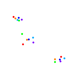
Superimposing all the images, the misalignment is clear:

The coordinates of the landmarks are stored in a point file in the Elastix format, with the points sorted according to the criterion discussed previously:

index
18
61	58	0
94	129	0
196	195	0
57	65	1
108	123	1
211	191	1
62	67	2
72	111	2
180	203	2
71	64	3
109	139	3
198	201	3
44	55	4
75	145	4
200	186	4
50	60	5
88	130	5
180	194	5

Elastix requires at least one ImageToImageMetric to be present in order to run. For this reason, to test the groupwise point metric we need to add a dummy intensity metric, setting its weight to zero so it will not affect the registration process. Here I use the AdvancedMeanSquares, since it is cheap to compute. A gray scale version of the images, packed in a 3D volume, is used as input. The parameter file looks like the following:

(Registration "MultiMetricMultiResolutionRegistration")
(Interpolator "ReducedDimensionBSplineInterpolator")
(ResampleInterpolator "FinalReducedDimensionBSplineInterpolator")
(BSplineInterpolationOrder 1)
(FinalBSplineInterpolationOrder 3)
(Transform "BSplineStackTransform")
(HowToCombineTransforms "Compose")

(Optimizer "AdaptiveStochasticGradientDescent")
(NumberOfSpatialSamples 2000)
(ImageSampler "RandomCoordinate")

(FinalGridSpacingInPhysicalUnits 20)
(Metric "AdvancedMeanSquares" "CorrespondingPointsMeanDistanceMetric")

(Metric0Weight 0.0)
(Metric1Weight 1.0)

(MovingImageDerivativeScales 1 1 0)

(NumberOfResolutions 1)
(MaximumNumberOfIterations 1000)

Setting the MovingImageDerivativeScales parameter equal to zero on the last dimension prevents movements along the time axis. We should also avoid setting a too small spline grid spacing in this example, since the transform has no regularisation.

After unpacking the output volume and colouring back the images, the result looks like the following:

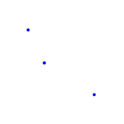
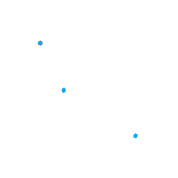
We can superimpose the output images (here in black) together with the input images (in colour):

Source code

The complete implementation of this metric is available on GitHub. Enjoy!

References

1. C. T. Metz, S. Klein, M. Schaap, T. van Walsum, and W. J. Niessen, “Nonrigid registration of dynamic medical imaging data using nD+ t B-splines and a groupwise optimization approach,” Medical image analysis, vol. 15, no. 2, pp. 238–249, 2011.
2. W. Huizinga et al., “PCA-based groupwise image registration for quantitative MRI,” Medical image analysis, vol. 29, pp. 65–78, 2016.
3. S. Klein, M. Staring, K. Murphy, M. A. Viergever, and J. P. W. Pluim, “Elastix: A toolbox for intensity-based medical image registration,” IEEE transactions on medical imaging, vol. 29, no. 1, pp. 196–205, 2010.
4. S. Klein, J. P. W. Pluim, M. Staring, and M. A. Viergever, “Adaptive stochastic gradient descent optimisation for image registration,” International journal of computer vision, vol. 81, no. 3, p. 227, 2009.
5. F. Wang, B. C. Vemuri, A. Rangarajan, and S. J. Eisenschenk, “Simultaneous nonrigid registration of multiple point sets and atlas construction,” IEEE transactions on pattern analysis and machine intelligence, vol. 30, no. 11, pp. 2011–2022, 2008.
6. T. Chen, B. C. Vemuri, A. Rangarajan, and S. J. Eisenschenk, “Group-wise point-set registration using a novel CDF-based Havrda-Charvát divergence,” International journal of computer vision, vol. 86, no. 1, p. 111, 2010.

Footnotes