Visualisation is a complementary but very important part of my work on image analysis. And since I work mainly with tridimensional volume images, visualisation is inherently a more complicated task compared to image analysis in only two dimensions. To help my work, I decided to implement a small tool for volumetric rendering, aimed to be minimal and very lightweight, fast, and easy to extend.
One may wonder why to start a new tool from scratch, when quite good options for scientific visualisation are already available, for instance ParaView or 3D Slicer. The answer is that those tools, despite being feature-rich, are slow, heavy, and non-trivial to extend. On the other hand, what I would like to have is a bare-bone, very lightweight tool, that allows me to write and use custom shaders and possibly CUDA kernels to directly operate on the volumes GPU-side. This tool aims to be a sort of simple application skeleton that can be easily customised as needed.
Given these requisites, C++ is a reasonable language option, and the toolkit of choice for this project is Qt, which is very complete and feature-rich, but at the same time simple to use, and it comes with a fairly good IDE, QtCreator. It also offers a reasonably good OpenGL interface, allowing to easily integrate an OpenGL canvas within an application.
The principles of raycasting

Raycasting is a visualisation technique for volume rendering. In a nutshell, it consists of casting rays from the camera through each pixel of the viewport. Each ray draws a path through the volume, and intensity samples are collected along this path and used to render the pixel corresponding to the ray.
Given a volume, in order to perform raycasting we need to cast a ray for each pixel in the viewport, and for each ray we need to determine the coordinates of its entry and exit points with respect to the volume. Once these two points are known, it is trivial to sample the volume and use the collected values to perform shading.
Two-pass raycasting
The simplest technique for volumetric raycasting is the so-called two-pass raycasting. The name comes from the fact that rendering is performed in two GPU passes: a first pass to compute the bounding geometry, i.e. the entry and exit points of the rays generated by each pixel in the viewport, rendering them to a couple of textures, and a second pass to perform the actual sampling and shading.
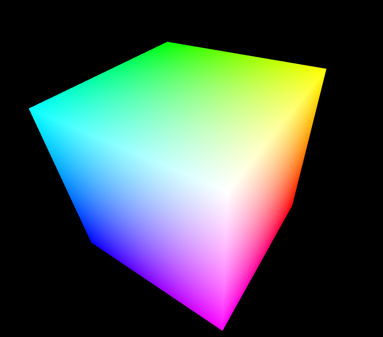
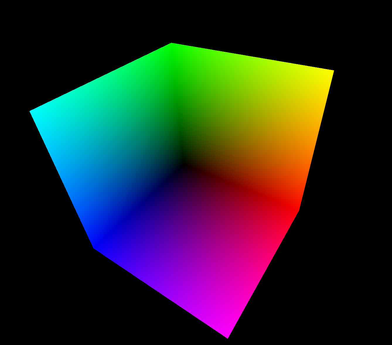
In the first pass, the trick is to render to a framebuffer the bounding box of the volume, defined as a two-unit cube. A model transform will compensate for differences in size among the axes, anisotropy, and spatial orientation. The framebuffer will have two colour attachments bound to it: one will collect the spatial coordinates of the entry points, given by the front-face of the cube, the other will collect the exit points, given by the back-face. This can be easily achieved by applying the desired model-view-projection transform in the vertex shader, while passing to the fragment shader the non-transformed coordinates of the vertex. A very simple fragment shader allows to store them in the correct texture of the framebuffer, according to whether the fragment belongs to a front face or not, and performs a conversion from two-unit cube coordinates (range \([-1, 1]\)) to texture coordinates (range \([0, 1]\)).
#version 130

in vec3 position;
out vec3 start_point;
out vec3 end_point;

void main()
{
    if (gl_FrontFacing) {
        start_point = 0.5 * (position + 1.0);
        end_point = vec3(0);
    } else {
        start_point = vec3(0);
        end_point = 0.5 * (position + 1.0);
    }
}
For this to work, it is necessary to enable GL_BLEND before rendering the
cube, and use two render targets, one for each attachment:
glEnable(GL_BLEND);
glBlendFunc(GL_ONE, GL_ONE);
GLenum renderTargets[2] = {GL_COLOR_ATTACHMENT0, GL_COLOR_ATTACHMENT1};
glDrawBuffers(2, &renderTargets[0]);
The resulting textures will look more or less like this:
Once the entry and exit points are computed, we are ready for the second pass. This time we will render a full-screen quad, binding the entry and exit points to a couple of texture units. For each fragment we will sample the entry and exit points, compute the ray direction, given by their difference, and gather samples along the path of the ray through the volume. We set a step length defining the distance between the samples, whose value offers a compromise between quality and speed: a large step length gives a fast computation with a poor quality result, and vice versa a small step length has a high cost but produces a better result.
Since we are rendering a full-screen quad, some rays may not intersect the volume at all. We can easily recognise and discard them. Since we are sampling from already discretised data, it is a good idea to apply a stochastic jitter to the starting position of the ray, that we can compute on the CPU as random noise and pass to the GPU in a texture, in order to reduce wood grain artifacts.
void main()
{
    vec3 ray_start = texture(front_face, fragment_coordinates).xyz;
    vec3 ray_stop = texture(back_face, fragment_coordinates).xyz;

    if (ray_start == ray_stop) {
        discard;
        return;
    }

    vec3 ray = ray_stop - ray_start;
    float ray_length = length(ray);
    vec3 step_vector = step_length * ray / ray_length;

    // Random jitter
    ray_start += step_vector * texture(jitter, fragment_coordinates).r;

    vec3 position = ray_start;

    // Stop when the end of the volume is reached
    while (ray_length > 0) {

        float intensity = texture(volume, position).r;

        // Do something with the sample
        // ...

        ray_length -= step_length;
        position += step_vector;
    }
}
Single-pass raycasting
While being very simple to implement, two-pass raycasting is suboptimal. Apart from the obvious overhead of two rendering passes, during the second pass we need two texture samplings, which are not cheap operations, just to recover the entry and exit points. Moreover, due to the full-screen quad rendering, it is not easy to integrate the volume rendering within a larger scene containing other objects. To overcome all these drawbacks, we can however perform volumetric raycasting in a single pass. A nice introduction to the topic is given in this post by Philip Rideout.
This time we will render the bounding geometry of the volume, which is still a two-unit cube, and compute the ray entry and exit points directly in the fragment shader, just before performing the actual shading. In order to do this, we need to pass to the shader a little more information, given by the camera position (in model coordinates) and field of view.

Given this information and knowing the normalised fragment coordinates (in range \([-1, 1]\)), we can easily write the parametric equation of the ray
\[\boldsymbol{p} = \boldsymbol{o} + t \boldsymbol{v}\]where \(\boldsymbol{o}\) is the origin of the ray, given by the position of the camera, and \(\boldsymbol{v}\) is its direction, given by the vector going from the camera to the fragment. The \(x\) and \(y\) coordinates of \(\boldsymbol{v}\) are given by the normalised coordinates of the fragment (correcting by the aspect ratio if the viewport is not a square), while its \(z\) coordinate is equal in absolute value to the focal length \(f\), that can be immediately computed from the field of view \(\alpha\) as
\[f = \frac{1}{\tan{\frac{\alpha}{2}}}\]Once we know the parametric equation of the ray, computing its intersections with the volume bounding box is an easy to solve geometric problem, since we are dealing with an axis-aligned bounding box (AABB). We can express the AABB with two triples, containing the intercepts of the top and bottom bounding planes orthogonal to each axis, and the intersections can be quickly computed with the slab method, which returns the parameter \(t\) for the near and far intersection points. Note how we clamp to zero the parameter for the near intersection, since we are not interested into negative values, that correspond to positions behind the camera.
// Slab method for ray-box intersection
void ray_box_intersection(Ray ray, AABB box, out float t_0, out float t_1)
{
    vec3 direction_inv = 1.0 / ray.direction;
    vec3 t_top = direction_inv * (box.top - ray.origin);
    vec3 t_bottom = direction_inv * (box.bottom - ray.origin);
    vec3 t_min = min(t_top, t_bottom);
    vec2 t = max(t_min.xx, t_min.yz);
    t_0 = max(0.0, max(t.x, t.y));
    vec3 t_max = max(t_top, t_bottom);
    t = min(t_max.xx, t_max.yz);
    t_1 = min(t.x, t.y);
}
At this point, the fragment shader continues in a way similar to the two-pass case. Note that we do not need to check for rays that do not intersect the volume anymore, since this time we are rendering the bounding box itself, so we already know that all the fragments processed by the shader define rays passing through the volume.
void main()
{
    vec3 ray_direction;
    ray_direction.xy = 2.0 * gl_FragCoord.xy / viewport_size - 1.0;
    ray_direction.x *= aspect_ratio;
    ray_direction.z = -focal_length;
    ray_direction = (vec4(ray_direction, 0) * ViewMatrix).xyz;

    float t_0, t_1;
    Ray casting_ray = Ray(ray_origin, ray_direction);
    AABB bounding_box = AABB(top, bottom);
    ray_box_intersection(casting_ray, bounding_box, t_0, t_1);

    vec3 ray_start = (ray_origin + ray_direction * t_0 - bottom) / (top - bottom);
    vec3 ray_stop = (ray_origin + ray_direction * t_1 - bottom) / (top - bottom);

    vec3 ray = ray_stop - ray_start;
    float ray_length = length(ray);
    vec3 step_vector = step_length * ray / ray_length;

    // Random jitter
    ray_start += step_vector * texture(jitter, gl_FragCoord.xy / viewport_size).r;

    vec3 position = ray_start;

    // Stop when the end of the volume is reached
    while (ray_length > 0) {

        float intensity = texture(volume, position).r;

        // Do something with the sample
        // ...

        ray_length -= step_length;
        position += step_vector;
    }
}
Rendering techniques
Now that we have a mechanism to sample the volume, we can use such samples to perform the actual shading. There are different raycasting techniques that can be used, according to what we want to visualise, and that produce very different results.
Isosurface rendering
It is possible to visualise an isosurface extracted from the volume data, defined as the surface of the level set for a given threshold value. To perform isosurface extraction in our shader, we let the ray advance through the volume until we reach a sample whose intensity is greater or equal to the threshold value, meaning that we have hit the isosurface.
Generally speaking, isosurfaces extracted from volume data tend to be quite noisy and irregular so, in order to obtain a smoother result, we can refine it by bisecting the step length, searching for a sample point with intensity closer to the threshold within half step length from the point that hit.
Once we find a point belonging to the isosurface, it is possible to apply an illumination model to perform shading. One of the simplest is the Blinn-Phong illumination model, which defines the outgoing light as the sum of ambient, diffuse, and specular components. In order to apply the Blinn-Phong model, we need to know the normal of the surface at the point. This can be easily approximated by the gradient of the intensity at the current sample point, at the cost of three texture samplings, given that the data is reasonably continuous.
// Estimate the normal from a finite difference approximation of the gradient
vec3 normal(vec3 position, float intensity)
{
    float d = step_length;
    float dx = texture(volume, position + vec3(d,0,0)).r - intensity;
    float dy = texture(volume, position + vec3(0,d,0)).r - intensity;
    float dz = texture(volume, position + vec3(0,0,d)).r - intensity;
    return -normalize(NormalMatrix * vec3(dx, dy, dz));
}
Once the normal is computed, we have all the information we need to compute the illumination. The ray march loop in the fragment shader will look like this:
while (ray_length > 0) {

    float intensity = texture(volume, position).r;

    if (intensity > threshold) {

        // Get closer to the surface
        position -= step_vector * 0.5;
        intensity = texture(volume, position).r;
        position -= step_vector * (intensity > threshold ? 0.25 : -0.25);
        intensity = texture(volume, position).r;

        // Compute the local vectors
        vec3 L = normalize(light_position - position);
        vec3 V = -normalize(ray);
        vec3 N = normal(position, intensity);
        vec3 H = normalize(L + V);

        // Blinn-Phong shading
        float Id = kd * max(0, dot(N, L));
        float Is = ks * pow(max(0, dot(N, H)), specular_power);
        colour = (ka + Id) * material_colour + Is * specular_colour;

        break;
    }

    ray_length -= step_length;
    position += step_vector;
}
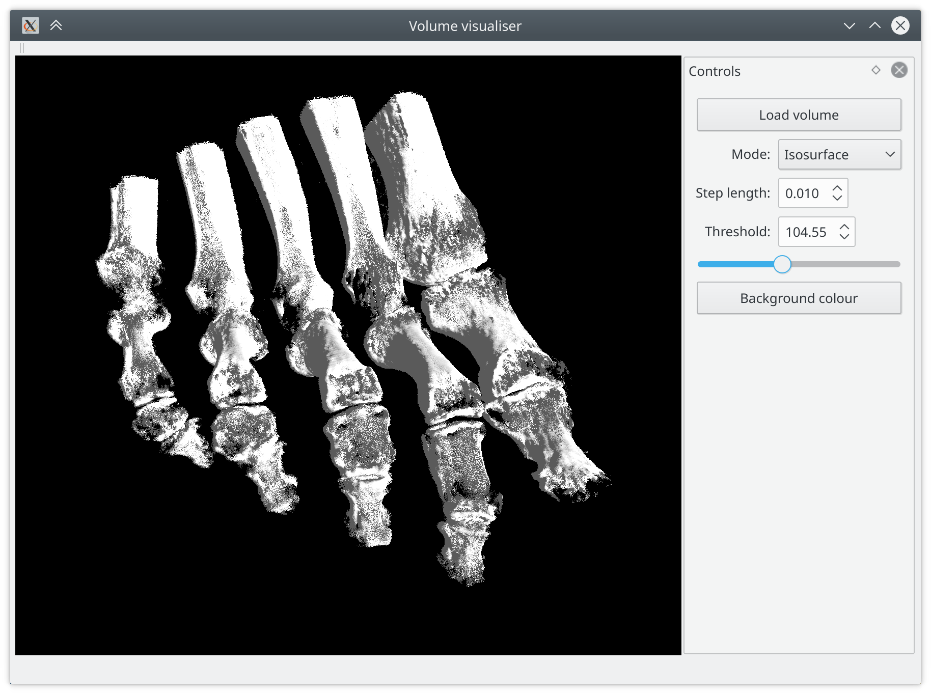
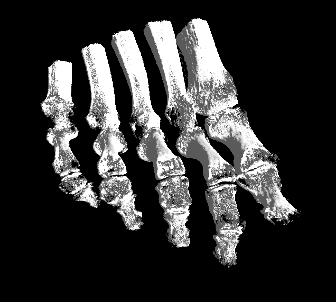
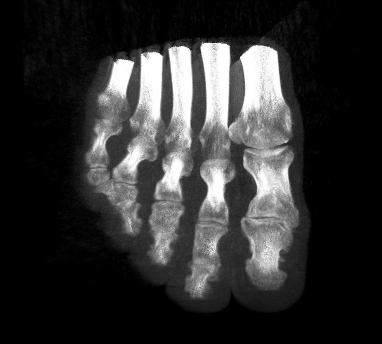
This technique is well suited to visualise the skeleton from CT data, since the bones have a significantly higher radiodensity compared to other tissues, giving them a generally good contrast in terms of Hounsfield units.
Maximum intensity projection
A very simple, yet surprisingly effective technique for volume rendering is called maximum intensity projection (MIP). In its simplest form, it consists of taking as intensity for the current fragment the maximum intensity sampled along the ray.
float maximum_intensity = 0.0; // Assuming intensity in [0, 1]

// Stop when the end of the volume is reached
while (ray_length > 0) {

    float intensity = texture(volume, position).r;

    if (intensity > maximum_intensity) {
        maximum_intensity = intensity;
    }

    ray_length -= step_length;
    position += step_vector;
}
This technique works well to visualise a volume where inner regions have generally higher intensities compared to outer regions, and once again CT data is a good candidate, while for example most types of MR images will not look very interesting when taking the MIP.
Front-to-back alpha-blending
This is probably the most versatile technique, and it allows to produce the most complex results, but at the same time it requires more work, and the settings are generally tied to the type of image to visualise.
The principle is to use a transfer function to map intensity values to colours, and perform front-to-back alpha blending of the samples acquired along the ray. One important reasons to render front-to-back is that it allows early stopping of the sampling when the colour of the fragment is saturated.
vec4 colour = vec4(0.0);

// Stop when the end of the volume is reached or the pixel is saturated
while (ray_length > 0 && colour.a < 1.0) {

    float intensity = texture(volume, position).r;
    float gradient = gradient_magnitude(position, intensity);

    vec4 c = colour_transfer(intensity);

    // Alpha-blending
    colour.rgb = c.a * c.rgb + (1 - c.a) * colour.a * colour.rgb;
    colour.a = c.a + (1 - c.a) * colour.a;

    ray_length -= step_length;
    position += step_vector;
}
We can also use gradient information to control the opacity of the samples, which is especially useful if we want to emphasise surfaces.
float gradient_magnitude(vec3 position, float intensity)
{
    float d = step_length;
    float dx = texture(volume, position + vec3(d,0,0)).r - intensity;
    float dy = texture(volume, position + vec3(0,d,0)).r - intensity;
    float dz = texture(volume, position + vec3(0,0,d)).r - intensity;
    return sqrt(dx * dx + dy * dy + dz * dz);
}
While the alpha blending code seems very easy so far, the tough part is to actually implement the colour transfer function. There is no general recipe for it, since it is very dependent upon the type of data to be visualised, and on which features of the data should be emphasised. One of the simplest meaningful transfer functions interpolates between a couple of colours denoting minimum and maximum intensity. For example, using exponential decay for the opacity and a gradient-based attenuation factor:
// A very simple colour transfer function
vec4 colour_transfer(float intensity, float gradient)
{
    vec3 high = vec3(1.0, 1.0, 1.0);
    vec3 low = vec3(0.0, 0.0, 0.0);
    float alpha = (exp(ki * intensity) - 1.0) / (exp(ki) - 1.0);
    alpha *= 1.0 - 1.0 / (1.0 + kg * gradient);
    return vec4(intensity * high + (1.0 - intensity) * low, alpha);
}
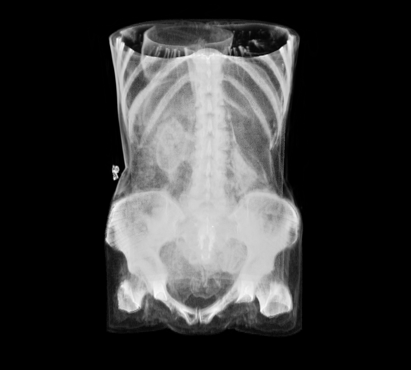
If we use this function to render a CT volume, we obtain something like the following, where it is possible to see the dimmed outlines of tissues, organs, and main vessels:
Adding a GUI
As mentioned in the beginning, to implement a simple and handy tool we can add a Qt GUI to provide an interface to the visualiser. The key class is QOpenGLWidget, that allows to render OpenGL content and can be used to implement a canvas for the raycasting. Inheriting from QOpenGLExtraFunctions allows to call OpenGL functions as class members and simplifies context handling.
Some key virtual member functions that we want to override are
initializeGL(), that will contain all OpenGL-related initialisation,
paintGL(), which will render a single frame, and resizeGL(), which will
handle window resizing.
class RayCastCanvas : public QOpenGLWidget, protected QOpenGLExtraFunctions
{
    Q_OBJECT
public:
    explicit RayCastCanvas(QWidget *parent = nullptr);
    ~RayCastCanvas();

    // ...

protected:
    void initializeGL();
    void paintGL();
    void resizeGL(int width, int height);

    // ...
};
I also defined a handful of helper classes to model objects: RayCastVolume,
holding the state of a volume object that we want to render, and Mesh,
representing a triangle mesh (such as the bounding box of the volume). Once
again, by inheriting from QOpenGLExtraFunctions, we can implement within a
paint() member the logic required by an object to render itself.
class RayCastVolume : protected QOpenGLExtraFunctions
{
public:
    RayCastVolume(void);
    virtual ~RayCastVolume();

    void paint(void);

    // ...
};

class Mesh : protected QOpenGLExtraFunctions
{
public:
    Mesh(const std::vector<GLfloat>& vertices, const std::vector<GLuint>& indices);
    virtual ~Mesh();

    void paint(void);

    // ...
};
The Qt example applications include a nice implementation of a trackball, available under the BSD license, that we can include to allow rotating the volume with the mouse. I also implemented a small reader that allows to open volumes from files in the VTK structured points legacy format. With Qt Designer we can easily set up the main window and a docking widget containing some controls. This already gives us a nice skeleton application, that can be very easily extended in a modular way. The complete source code is available on GitHub. Enjoy!